Array Operations and Broadcasting

Element-wise Operations: The Basics

The simplest operations in NumPy are element-wise. This means that when you perform an operation like addition between two arrays, the operation is applied to each pair of corresponding elements.

Operations Between Arrays of the Same Shape

When two arrays have the exact same shape, arithmetic operations are straightforward. The operation is applied element by element.

import numpy as np

# Create two 2x3 arrays
a = np.array([[1, 2, 3], 
              [4, 5, 6]])

b = np.array([[10, 10, 10], 
              [20, 20, 20]])

# Element-wise addition
print("a + b =")
print(a + b)

# Element-wise multiplication
print("\na * b =")
print(a * b)

The result is a new array of the same shape, where each element is the result of the operation on the elements from a and b at that same position.

Operations with a Scalar

What happens when you try to operate on an array and a single number (a scalar)? NumPy handles this gracefully using the simplest form of broadcasting. It effectively "stretches" the scalar to match the shape of the array.

a = np.array([1, 2, 3])

# Add a scalar to an array
print(a + 5)  # Output: [6 7 8]

# Multiply an array by a scalar
print(a * 10) # Output: [10 20 30]

Conceptually, NumPy treats the scalar 5 as an array [5, 5, 5] to perform the element-wise addition. This is done without actually creating a new array in memory, which is why it's so efficient.

To see these basic operations in action, the following video provides a clear introduction.

Broadcasting: The Core Idea

Broadcasting is the powerful mechanism that generalizes the scalar-array operation. It allows NumPy to perform universal functions (like addition, multiplication, etc.) on arrays of different, but compatible, sizes.

Let's start by reading a concise introduction to the concept.

As the text explains, we can think of broadcasting as a way of stretching arrays so they have a common shape, allowing for element-wise operations.

The Rules of Broadcasting

For broadcasting to work, NumPy follows a strict algorithm to check if two arrays are compatible. This check proceeds from the trailing (i.e., rightmost) dimensions.

The three rules of broadcasting are:

1. Rule 1: If the two arrays differ in their number of dimensions, the shape of the one with fewer dimensions is padded with ones on its leading (left) side.
2. Rule 2: If the shape of the two arrays does not match in any dimension, the array with a shape equal to 1 in that dimension is "stretched" to match the other shape.
3. Rule 3: If in any dimension the sizes disagree and neither is equal to 1, an error (ValueError) is raised.

To truly internalize these rules, let's watch a video that explains them in detail with clear examples.

Walking Through an Example

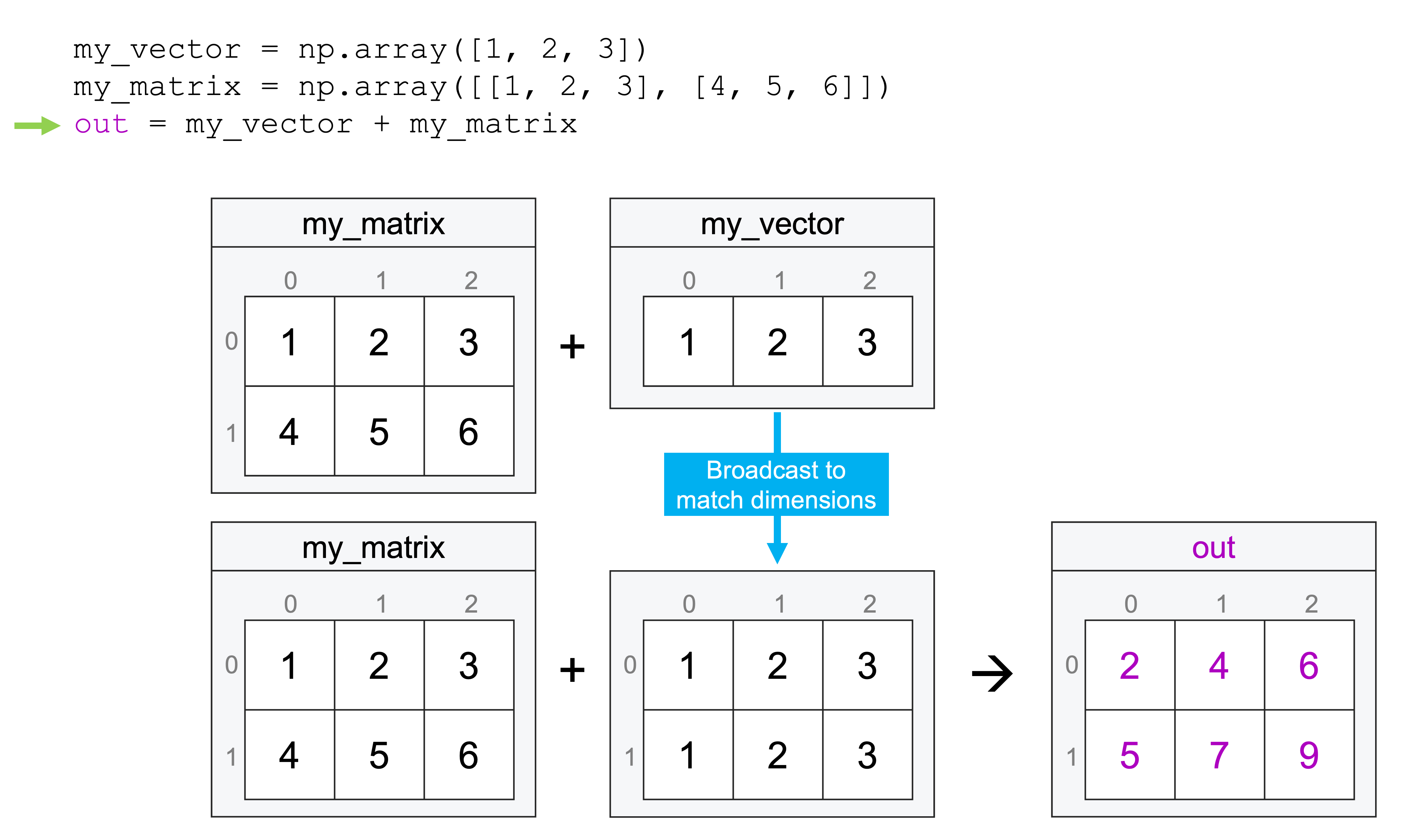
Let's apply these rules manually to an example. Imagine we want to add a 1D array to a 2D array.

# A 2x3 matrix
M = np.ones((2, 3))  # Shape: (2, 3)

# A 1D vector
a = np.arange(3)     # Shape: (3,)

result = M + a

Here's how NumPy processes this:

1. Initial Shapes:

   • M.shape = (2, 3)
   • a.shape = (3,)

2. Apply Rule 1: Array a has fewer dimensions. We pad its shape on the left with a 1.

   • M.shape -> (2, 3)
   • a.shape -> (1, 3)

3. Apply Rule 2: We compare the shapes dimension by dimension, from right to left.

   • Trailing dimension: Both are 3. They match.
   • Leading dimension: M has 2, a has 1. Since a's dimension is 1, it is "stretched" to match M's dimension of 2.

4. Final (virtual) Shapes: Both arrays are now compatible with a shape of (2, 3). The operation proceeds.

Broadcasting in Practice: Centering Data

Broadcasting isn't just a theoretical curiosity; it's at the core of many data science tasks. A common preprocessing step in machine learning is to center data by subtracting the mean of each feature (column) from the dataset.

Imagine you have a dataset of 10 samples, each with 3 features, stored in a 10x3 array.

# Generate some random data: 10 samples, 3 features
X = np.random.random((10, 3))

# 1. Calculate the mean of each feature (column)
# axis=0 means we compute the mean down the columns
X_mean = X.mean(axis=0)

print(f"Shape of our data X: {X.shape}")
print(f"Shape of our means X_mean: {X_mean.shape}\n")

# 2. Center the data by subtracting the mean
# This is a broadcasting operation!
X_centered = X - X_mean

print(f"Shape of the centered data: {X_centered.shape}")

# To verify, the mean of the centered data should be very close to zero
print(f"\nNew column means:\n{X_centered.mean(axis=0)}")

In the line X - X_mean, NumPy broadcasts the (3,) mean array across the (10, 3) data array, subtracting the correct column mean from every row. Without broadcasting, you would need to write a manual loop, which is both slower and more verbose in Python.

This specific application and others are demonstrated in the following article.

Conclusion

In this lesson, we demystified how NumPy performs operations on arrays, especially when their shapes differ. This is a fundamental concept that you will use constantly as you progress.

Key Takeaways:

• Element-wise operations apply an operator to corresponding elements of arrays that have the same shape.
• Broadcasting is the set of rules NumPy uses to perform operations on arrays of different but compatible shapes, avoiding slow Python loops.
• Broadcasting compatibility is determined by three rules that compare array shapes from right to left, padding and stretching dimensions where possible.
• A common practical application is vectorizing operations like centering data, where you subtract a 1D mean array from a 2D data matrix.

Preview of the Next Lesson:
Now that you can create, reshape, and perform calculations on arrays, the next step is to master how to select specific data from them. In the next lesson, we will cover advanced indexing, slicing, and boolean masking, which allow you to filter and retrieve array elements based on complex conditions. This is a crucial skill for any form of data analysis.