Array Indexing, Slicing, and Boolean Masking

1. Basic Indexing and Slicing

Just like with Python lists, you can access and manipulate parts of a NumPy array using index notation. However, NumPy extends this capability in powerful ways for multi-dimensional arrays.

1D Arrays: A Familiar Start

For one-dimensional arrays, indexing and slicing work almost exactly as they do with Python lists.

• arr[i] accesses the element at index i.
• arr[start:stop] extracts a range of elements.
• arr[start:stop:step] extracts elements with a specific step.

import numpy as np

arr_1d = np.arange(10) # array([0, 1, 2, 3, 4, 5, 6, 7, 8, 9])

# Access a single element
print(f"Element at index 3: {arr_1d[3]}")

# Slice from index 2 up to (but not including) index 5
print(f"Slice from 2 to 5: {arr_1d[2:5]}")

# Get every other element from the start to the end
print(f"Every other element: {arr_1d[::2]}")

2D Arrays: Rows and Columns

For multi-dimensional arrays, NumPy provides a more intuitive and efficient syntax. Instead of chaining brackets like arr[row][column], you use a single pair of brackets with comma-separated indices: arr[row, column].

• arr[row, col]: Access a single element.
• arr[row, :]: Access an entire row.
• arr[:, col]: Access an entire column.
• arr[r_start:r_stop, c_start:c_stop]: Access a sub-array or "sub-matrix".

The following image provides an excellent visual guide to these operations.

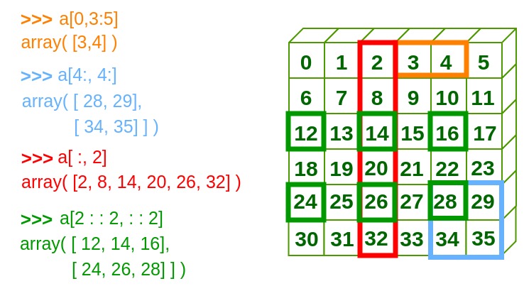
To see these concepts in action and understand how to apply them to arrays with 1, 2, and even 3 dimensions, the following video provides a clear, hands-on demonstration.

2. An Important Distinction: Views vs. Copies

This is a key concept that addresses the "why" behind NumPy's behavior. When you slice an array, does it create a new, independent array in memory, or does it just create a "view" into the original array?

• Basic Slicing creates a view: When you use basic slicing (like arr[0:5] or arr[:, 1]), NumPy does not create a new array. It gives you a view into the original array's data. This is extremely memory-efficient. The consequence is that if you modify the slice, you also modify the original array.
• Advanced or "Fancy" Indexing creates a copy: When you index using a list of integers (e.g., arr[[0, 2, 4]]), you are performing "fancy" indexing. This operation always creates a new array with a copy of the data. Modifying this new array will not affect the original.

To understand this crucial difference, let's read a short section from a very well-regarded technical blog.

subset_a = data[2:5]
subset_a[0] = 99

data = np.arange(10) # Reset the array
subset_b = data[[2, 3, 4]]
subset_b[0] = 99

3. Boolean Masking

Boolean masking is perhaps the most powerful indexing technique for data analysis. It allows you to select elements from an array based on a condition. The process involves two steps:

1. Create a boolean mask: This is an array of True/False values that has the same shape as your data array. You create it by applying a condition directly to the array.
2. Apply the mask: Use the boolean mask as the index to your data array. This will return a 1D array containing only the elements where the mask was True.

data = np.array([[1, 2], [3, 4], [5, 6]])

# 1. Create a boolean mask
mask = data > 3
print("Boolean mask:\n", mask)
# [[False, False],
#  [False,  True],
#  [ True,  True]]

# 2. Apply the mask to the data
print("\nElements where data > 3:", data[mask]) # Output: [4 5 6]

Boolean masking is a form of fancy indexing, so it returns a copy of the data, not a view.

Combining Conditions

You can create more complex masks by combining conditions using bitwise operators:

• & for AND
• | for OR
• ~ for NOT

Important: When combining conditions, you must wrap each condition in parentheses due to Python's operator precedence rules. For example: (data > 2) & (data < 5).

The next video segment demonstrates how to use boolean masking and combine multiple conditions to filter your data effectively.

You can also use a boolean mask to modify values in the original array. This is a very common pattern for data cleaning.

temps = np.array([22.5, 25.0, -99.0, 23.1, 1000.0, 24.3])

# Create a mask for "impossible" temperatures
outlier_mask = (temps < -50) | (temps > 60)

# Use the mask to replace these values with NaN (Not a Number)
temps[outlier_mask] = np.nan

print(temps)
# Output: [22.5 25.   nan 23.1   nan 24.3]

Conclusion

Today, you've added some of the most essential NumPy skills to your toolkit. Being able to precisely select, filter, and modify data is a prerequisite for any serious data work.

Key Takeaways:

• Basic Indexing & Slicing: Use the [row, col] syntax for multi-dimensional arrays. Slicing with : lets you grab entire rows, columns, or sub-arrays.
• Views vs. Copies: Basic slicing creates memory-efficient views, where changes affect the original array. Fancy indexing (with lists) and boolean masking create independent copies.
• Boolean Masking: This powerful technique allows you to select and modify array elements based on one or more conditions (arr[condition]). Always use &, |, and () when combining conditions.

Preview of the Next Lesson:
Now that you know how to create, calculate with, and select from arrays, our next lesson will cover how to generate random data using NumPy's random module. This is a fundamental skill for creating sample datasets, initializing machine learning models, and performing statistical simulations.