Calculating Descriptive Statistics

1. Measures of Central Tendency: Finding the "Center"

When you get a new dataset, one of the first questions you'll ask is, "What does a typical value look like?" Measures of central tendency answer this question.

There are three common measures:

• Mean: The arithmetic average of all the data points.
• Median: The middle value when the data is sorted.
• Mode: The most frequently occurring value in the dataset.

The mean is the most common measure of center, but as you'll see, the median is more "robust" to extreme values or outliers. Since you have a strong background in programming, let's jump right into a practical explanation that uses the Pandas library you'll be working with extensively.

As the video explained, while the mean gives you the average, the median can often give you a better sense of the "typical" value in datasets with skewed distributions or extreme outliers (like house prices or salaries).

2. Measures of Spread: Variance and Standard Deviation

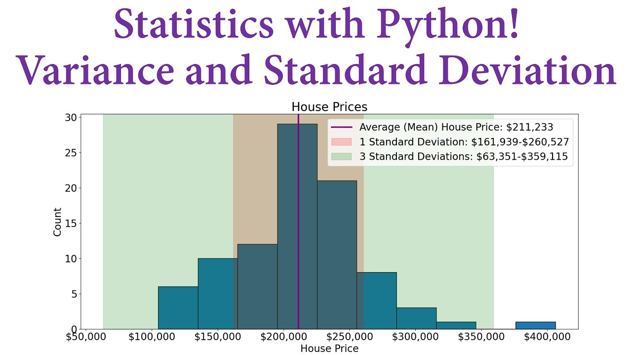
Knowing the center of the data is only half the story. We also need to know how spread out, or dispersed, the data is. Are all the data points clustered tightly around the mean, or are they scattered far and wide?

The Core Idea: Deviation from the Mean

To measure spread, we can calculate how far each data point $x_i$ is from the mean ($\bar{x}$). This is the deviation: $(x_i-\bar{x})$.

If we just averaged these deviations, the positive and negative values would cancel each other out, summing to zero. To solve this, we square each deviation, making them all positive: $(x_i-\bar{x}{)}^2$.

• Variance (${\sigma }^2$ or $s^2$): This is the average of the squared deviations. A larger variance means the data is more spread out.
• Standard Deviation ($\sigma$ or $s$): This is simply the square root of the variance. The key advantage is that it returns the measure of spread to the original units of the data, making it much more interpretable. For example, if you're measuring heights in centimeters, the standard deviation will also be in centimeters.

A Crucial Distinction: Population vs. Sample

This is one of the most important concepts in statistics.

• A population is the entire group you are interested in (e.g., all houses in a city).
• A sample is a smaller, manageable subset of that population (e.g., 1000 houses you collected data on).

In machine learning, we almost always work with samples. Our goal is to use the sample to estimate the characteristics of the entire population. This leads to a subtle but critical change in the formula for variance.

The following video provides an exceptionally clear explanation of this concept.

To summarize the key takeaway from Josh Starmer's video:

• When you have data for the entire population, you calculate variance by dividing the sum of squared differences by $n$.
• When you are using a sample to estimate the population's variance, you divide by $n-1$. This is known as Bessel's correction.

Since we're almost always working with samples in data science, the $n-1$ version is the one you will use most of the time.

3. Computing Descriptive Statistics in Python

Now, let's bring this theory into code. Your tools of choice, NumPy and Pandas, have this distinction built right in. The key is a parameter called ddof, which stands for "Delta Degrees of Freedom." It's the value you subtract from n in the denominator.

• ddof=0 means the denominator is $n$. Use this for population statistics.
• ddof=1 means the denominator is $n-1$. Use this for sample statistics.

The following guide shows you the exact syntax.

Here's a quick summary of the implementation. A crucial point to remember is that Pandas calculates sample statistics by default (ddof=1), which is usually what you want. NumPy defaults to population statistics (ddof=0).

import numpy as np
import pandas as pd

# Let's say this is a SAMPLE of data
data = [155, 160, 162, 175, 180] 

# --- Using NumPy ---
# You must specify ddof=1 for sample statistics
sample_std_np = np.std(data, ddof=1)
# The default is ddof=0 for population statistics
pop_std_np = np.std(data) # or np.std(data, ddof=0)

print(f"NumPy Sample Std Dev (n-1): {sample_std_np:.2f}")
print(f"NumPy Population Std Dev (n): {pop_std_np:.2f}")
print("-" * 20)

# --- Using Pandas ---
s = pd.Series(data)
# Pandas defaults to ddof=1 for sample statistics
sample_std_pd = s.std()
# To get population std dev, you must specify ddof=0
pop_std_pd = s.std(ddof=0)

print(f"Pandas Sample Std Dev (n-1): {sample_std_pd:.2f}")
print(f"Pandas Population Std Dev (n): {pop_std_pd:.2f}")

Practical Shortcut: .describe()

Calculating these one by one is good for learning, but for quick analysis, Pandas provides a wonderfully convenient method: .describe(). It computes all the key descriptive statistics for a Series or DataFrame in one go.

s = pd.Series(data)
print("\nPandas .describe() output:")
print(s.describe())

Notice the output includes the count, mean, std (standard deviation), min, max, and percentiles (like the median, which is the 50% mark).

Conclusion

You've just learned how to compute the most fundamental descriptive statistics, which form the bedrock of exploratory data analysis. These simple numbers can tell you a powerful story about your data's central tendency and spread.

Key Takeaways:

• Mean, Median, and Mode describe the center of your data. The mean is the average, while the median is more robust to outliers.
• Variance and Standard Deviation describe the spread or dispersion of your data around the mean. Standard deviation is often preferred because it's in the same units as the original data.
• The distinction between Population and Sample statistics is crucial. When estimating population metrics from a sample, you must use the $n-1$ denominator (Bessel's correction).
• In Python, you control this using the ddof parameter. Pandas defaults to ddof=1 (sample), while NumPy defaults to ddof=0 (population).
• The .describe() method in Pandas is your go-to for a quick statistical summary.

Preview of the Next Lesson:
We've introduced the important idea of populations and samples. In the next lesson, we will formalize this distinction. We'll explore what makes a good sample, the concept of sampling distributions, and why this is all so foundational for making inferences in machine learning.