Understanding Common Probability Distributions

1. What is a Probability Distribution?

A probability distribution is a function that provides the probabilities of occurrence of different possible outcomes in an experiment. Think of it as a complete map of a random phenomenon.

We can broadly classify distributions into two types:

• Discrete Distributions: The variable can only take on a countable number of distinct values. For example, the outcome of a dice roll (1, 2, 3, 4, 5, 6) or the number of heads in 10 coin flips.
• Continuous Distributions: The variable can take any value within a given range. For example, the height of a person or the temperature of a room.

Let's explore our first distribution, which is the simplest of them all.

2. The Uniform Distribution: All Outcomes are Equal

The uniform distribution is characterized by one simple rule: every possible outcome has an equal probability of occurring.

A classic example of a discrete uniform distribution is rolling a fair six-sided die. The probability of rolling a 1, 2, 3, 4, 5, or 6 is exactly the same: $1/6$.

However, in machine learning, we often deal with continuous uniform distributions. Imagine you have a program that generates a random number between 10 and 30. If any number in that range is equally likely to be chosen, this follows a continuous uniform distribution.

Let's watch a quick conceptual overview.

Visualizing the Uniform Distribution

For a continuous uniform distribution defined on an interval from $a$ to $b$, its graph is a simple rectangle.

• The base of the rectangle is the interval $(b-a)$.
• The height is constant across this interval and is $1/(b-a)$. This ensures that the total area under the curve is $(b-a)\times (1/(b-a))=1$, a fundamental rule for all probability distributions.

Python Implementation

Now, let's see how to work with this in Python. We can use the scipy.stats library, a powerful tool for statistical functions, to generate data from a uniform distribution and visualize it.

The following resource provides a tutorial on this. We'll focus on the Uniform Distribution section.

Let's break down the key piece of code from that tutorial:

from scipy.stats import uniform
import seaborn as sns

# Generate 10,000 random variates from a uniform distribution
# starting at 'loc' = 10, with a 'width' (scale) of 20.
# So, numbers will be between 10 and 10+20=30.
data_uniform = uniform.rvs(size=10000, loc=10, scale=20)

# Plot the distribution
ax = sns.distplot(data_uniform, bins=100)
ax.set(xlabel='Uniform Distribution', ylabel='Frequency')

Running this code produces a histogram that is roughly flat, resembling the rectangle we discussed.

3. The Binomial Distribution: A Story of Success and Failure

Next up is the binomial distribution. This is a discrete distribution that models the number of "successes" in a fixed number of independent trials, where each trial has only two possible outcomes (e.g., success/failure, heads/tails, win/lose).

Think about these scenarios:

• The number of heads you get after flipping a coin 10 times.
• The number of defective items in a batch of 50.
• The number of patients who recover after 20 receive a new drug.

These can all be modeled by a binomial distribution. The key conditions are:

1. A fixed number of trials ($n$).
2. Each trial is independent.
3. Each trial has only two outcomes.
4. The probability of success ($p$) is constant for each trial.

Let's watch a video that explains this using the coin flip experiment.

Python Implementation

The binomial distribution is defined by its parameters $n$ (number of trials) and $p$ (probability of success). In Python, we can again use scipy.stats to explore it.

Here is the essential code:

from scipy.stats import binom

# Generate data from a binomial distribution
# n=10 trials, p=0.8 probability of success, repeated 10,000 times
data_binom = binom.rvs(n=10, p=0.8, size=10000)

# Plot the distribution
ax = sns.distplot(data_binom, kde=False) # kde=False is good for discrete dists
ax.set(xlabel='Binomial Distribution', ylabel='Frequency')

If you were to run this code with p=0.5, the distribution would be symmetric around 5. Since p=0.8, the distribution is skewed to the left, with the peak around 8, which makes intuitive sense: if success is likely, we expect more successes.

4. The Normal Distribution: The Bell Curve

The normal distribution, also known as the Gaussian distribution or "bell curve," is arguably the most important probability distribution in statistics. It's a continuous distribution that arises everywhere in nature and data science. Heights, weights, measurement errors, and test scores often follow a normal distribution.

Its key characteristics are:

• It's symmetric around its mean.
• The mean, median, and mode are all equal.
• Its shape is determined by two parameters: the mean ($\mu$), which sets the center of the distribution, and the standard deviation ($\sigma$), which determines its spread or width.

To build a solid intuition for this, the StatQuest video is one of the best resources available.

The 68-95-99.7 Rule

A very useful property of the normal distribution is the empirical rule, or the "68-95-99.7 rule". This rule states:

• Approximately 68% of the data falls within 1 standard deviation of the mean ($\mu \pm \sigma$).
• Approximately 95% of the data falls within 2 standard deviations of the mean ($\mu \pm 2\sigma$).
• Approximately 99.7% of the data falls within 3 standard deviations of the mean ($\mu \pm 3\sigma$).

This rule is a great mental shortcut for quickly understanding the spread of normally distributed data.

Python Implementation

Finally, let's see how to generate and plot a normal distribution in Python.

The core Python code is very similar to what we've seen before:

from scipy.stats import norm

# Generate data from a normal distribution with mean=0 and stddev=1
data_normal = norm.rvs(size=10000, loc=0, scale=1)

# Plot the distribution
ax = sns.distplot(data_normal, bins=100)
ax.set(xlabel='Normal Distribution', ylabel='Frequency')

This generates the classic bell shape. By changing loc and scale, you can shift and stretch this curve just as described in the StatQuest video.

Visual Summary

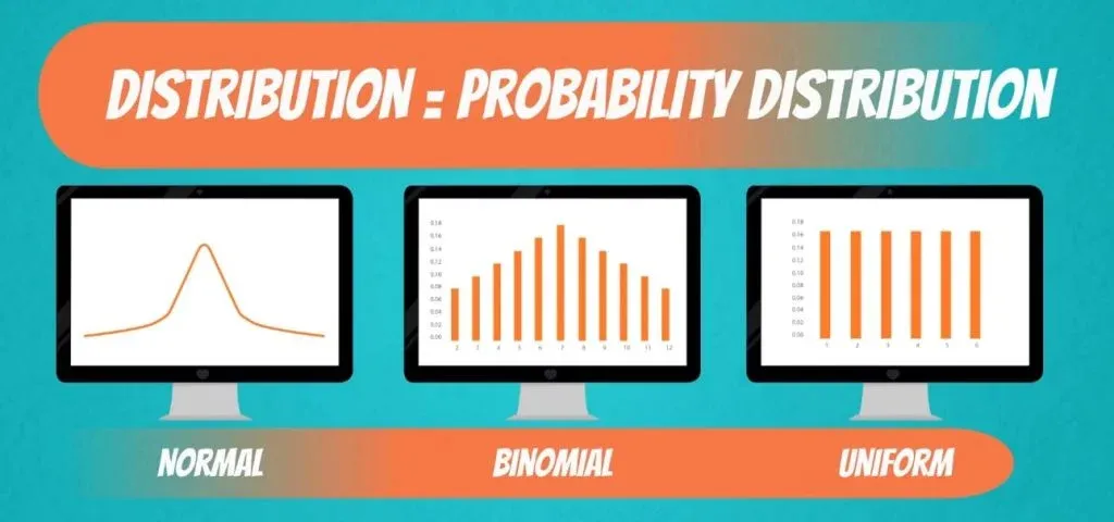
Here is a great image that shows the shapes of the three distributions we've discussed side-by-side. It's a useful visual reminder of their distinct characteristics.

Conclusion

In this lesson, we've moved from single probabilities to understanding the entire landscape of outcomes through probability distributions. These are essential tools for a data scientist.

Key Takeaways:

• Probability distributions describe the likelihood of all possible outcomes of a random variable.
• The Uniform Distribution models situations where all outcomes in a range are equally likely. It looks like a rectangle.
• The Binomial Distribution models the number of successes in a fixed number of discrete, independent trials. It's represented by bars.
• The Normal Distribution (or "bell curve") is a continuous distribution defined by its mean and standard deviation. It's symmetric and ubiquitous in real-world data.
• Libraries like scipy.stats and seaborn make it straightforward to work with and visualize these distributions in Python.

Preview of the Next Lesson:
We saw today that the normal distribution is defined by its mean and standard deviation. But how do we get those values from a set of data? In the next lesson, we will focus on descriptive statistics. You'll learn how to compute fundamental metrics like mean, variance, and standard deviation from a dataset, which are the first steps in summarizing and understanding any data you encounter.