Bayes' Theorem for Conditional Probability

1. From Probability to Conditional Probability

In the previous lesson, we asked questions like, "What is the probability of rolling a 7 with two dice?" Now, we'll ask a slightly different kind of question: "What is the probability that you rolled a 7, given that you know at least one of the dice is a 5?"

This "given that" part is the key. It means we have new information that changes the set of possible outcomes. The original sample space has been reduced. This new probability is called a conditional probability, denoted as $P(A|B)$, which reads "the probability of A given B".

The formal definition of conditional probability is:
$P(A|B)=\frac{P(A\cap B)}{P(B)}$
Where $P(A\cap B)$ is the probability that both A and B happen. In essence, we're restricting our universe to the outcomes where B is true, and then looking at the proportion of those outcomes where A is also true.

Let's watch a short video that derives this formula and then shows how it gives rise to Bayes' Theorem.

As you just saw, by writing out the definitions for $P(A|B)$ and $P(B|A)$ and noting that $P(A\cap B)$ is the same as $P(B\cap A)$, we can easily arrive at:

$P(A|B)=\frac{P(B|A)P(A)}{P(B)}$

This is Bayes' Theorem. It looks simple, but its implications are profound. It gives us a way to "flip" a conditional probability—if we know $P(B|A)$, we can find $P(A|B)$.

2. The Intuition: Updating Beliefs with Evidence

Before we dive into calculations, let's build a strong intuition for what Bayes' Theorem really does. It's a formal recipe for updating our beliefs. We start with an initial belief (a "prior") and, when we see new evidence, we update our belief to a new one (a "posterior").

There's no better way to understand this than with a classic thought experiment. The following video from 3Blue1Brown is one of the best explanations available.

The core takeaway is that our final belief shouldn't be based on the evidence alone. It should be a blend of our prior belief and the new evidence. The "Steve" example showed that even if the evidence strongly suggests "librarian," the low prior probability of being a librarian means the final answer might still be "farmer."

3. The Language of Bayes' Theorem

To apply the theorem effectively, we need to know the standard names for its components. This will help you map real-world problems onto the formula.

$\text{Posterior}=\frac{\text{Likelihood}\times \text{Prior}}{\text{Evidence}}$

Let's use a medical diagnosis example to make this concrete: "What is the probability a patient has cancer given a positive test result?"

• Posterior: $P(\text{Cancer | Positive})$
  This is what we want to calculate: the probability of having cancer after seeing the positive test result. It's our updated belief.

• Prior: $P(\text{Cancer})$
  This is our belief before seeing the evidence. It's the base rate or prevalence of cancer in the general population.

• Likelihood: $P(\text{Positive | Cancer})$
  This is the probability of seeing our evidence (a positive test) if our hypothesis is true (the patient has cancer). This is often related to the test's "sensitivity."

• Evidence: $P(\text{Positive})$
  This is the total probability of observing the evidence, regardless of whether the person has cancer or not. This is often the trickiest part to calculate.

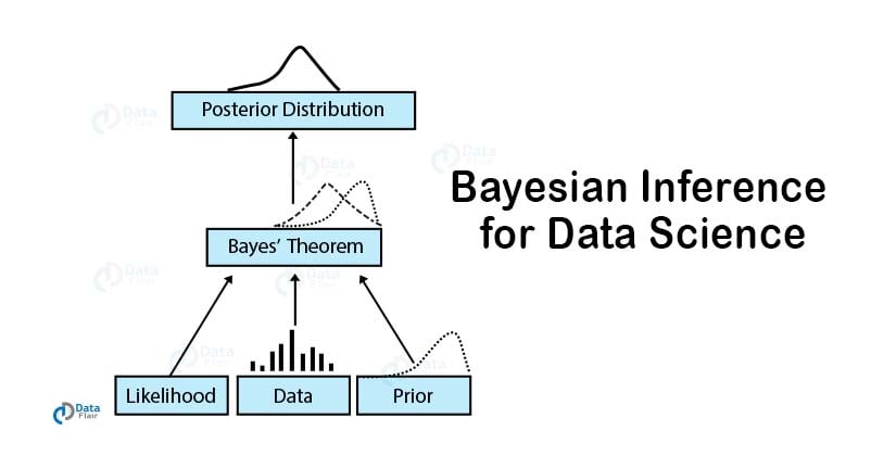
The following article provides a great summary of these terms and then dives into the classic medical diagnosis problem.

4. A Worked Example: The Deceptive Disease Test

Now let's put everything together with a full-fledged example. This problem is famous because the result is often surprisingly counter-intuitive and highlights a common statistical mistake known as the base rate fallacy.

Problem:
A disease has a prevalence of 1% in the population (our prior). A test for this disease has 95% accuracy:

• It correctly identifies 95% of sick people (true positive rate, our likelihood).
• It correctly identifies 95% of healthy people (true negative rate).

If a randomly selected person gets a positive test result, what is the probability they actually have the disease (the posterior)?

Most people's intuition says the probability should be around 95%. Let's see what Bayes' Theorem says.

To solve this, we first need to calculate the denominator, $P(\text{Positive})$. A positive result can happen in two ways:

1. A person has the disease AND tests positive (a true positive).
2. A person does NOT have the disease AND tests positive (a false positive).

We use the law of total probability to add these two mutually exclusive scenarios. A tree diagram is an excellent tool for visualizing this calculation.

Let's watch a video that solves a nearly identical problem using this method.

Now, let's see this same logic laid out in text and code. The article you looked at earlier provides a manual calculation and a Python function for a similar problem. Seeing the problem worked out in a different way will help solidify your understanding.

As you can see, the actual probability is much lower than 95%! This is because the base rate of the disease is so low that the number of false positives from the large healthy population outweighs the true positives from the small sick population. This is a critical lesson in data interpretation.

Conclusion

Today we've tackled one of the most important theorems in probability. You've seen how a simple rule for "flipping" conditional probabilities allows us to formalize the process of learning from data.

Key Takeaways:

• Conditional probability, $P(A|B)$, is the probability of event A happening given that event B has already occurred.
• Bayes' Theorem, $P(A|B)=\frac{P(B|A)P(A)}{P(B)}$, allows us to calculate a conditional probability when its "reverse" is known.
• The theorem is best understood as a way to update beliefs: we move from a prior belief to a posterior belief after observing evidence.
• Calculating the total probability of the evidence, $P(B)$, often requires breaking it down into all possible scenarios (e.g., using a tree diagram).
• Always be mindful of the base rate; ignoring it is a common and serious error in reasoning.

Preview of the Next Lesson:
So far, we've dealt with discrete events like coin flips and disease tests. But what about continuous measurements like height, temperature, or the price of a stock? In the next lesson, we will explore common probability distributions (like the Normal, Binomial, and Uniform distributions), which are the mathematical tools we use to model and understand both discrete and continuous random variables.