Gradient Boosting Classifier: Build and Evaluate

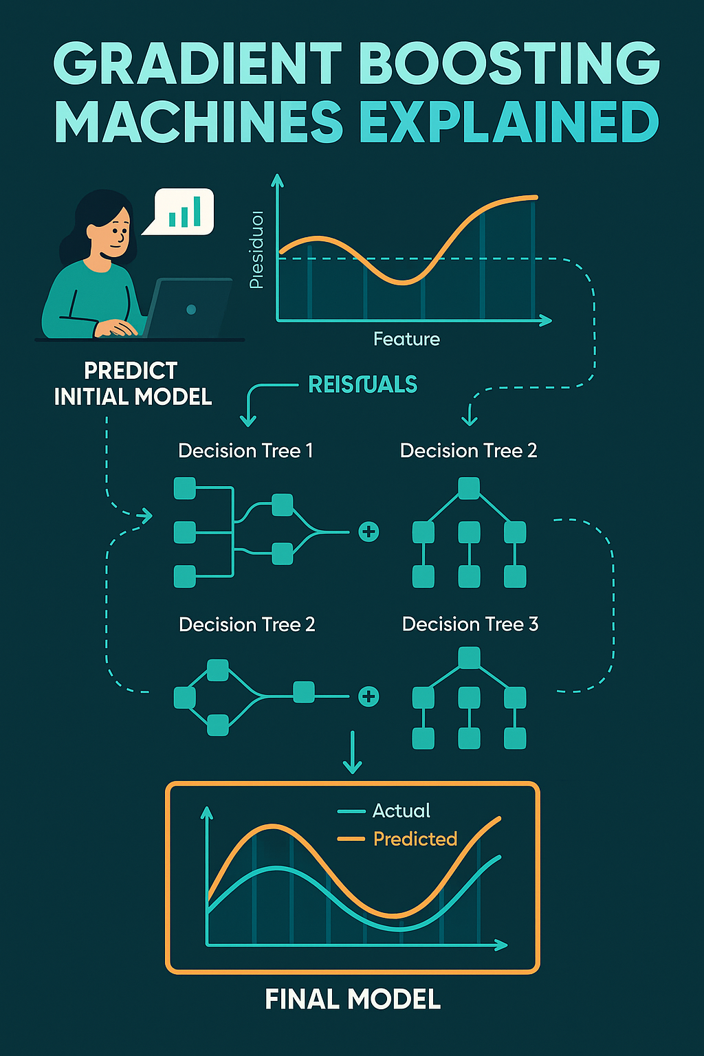
From Parallel to Sequential Learning

The fundamental difference between Random Forests and Gradient Boosting is how the ensemble is constructed.

• Random Forest (Parallel): Many independent trees are built on different subsets of data. They don't know about each other. Their collective vote determines the final prediction.
• Gradient Boosting (Sequential): Trees are built one after another. Each new tree is trained to correct the errors made by the combination of all previous trees.

This sequential approach is a form of boosting. Let's explore the intuition behind it.

The key steps you just read about are:

1. Initial Guess: Start with a simple prediction, typically the average of the target values (for regression) or the log-odds (for classification).
2. Calculate Residuals: Compute the errors made by the current model.
3. Fit a New Tree: Train a new, simple decision tree (a "weak learner") to predict these residuals. The idea is that this tree learns the patterns in the errors.
4. Update the Model: Add this new tree's predictions to the overall model, but scaled by a small factor called the learning rate.
5. Repeat: Go back to step 2 and repeat the process, fitting a new tree to the new residuals.

The "Gradient" in Gradient Boosting

So, where does the "gradient" part come from? The term "pseudo-residuals" is a clue. For certain loss functions, like Mean Squared Error (MSE), the residual (actual - predicted) is directly proportional to the negative gradient of the loss function.

Given your background in calculus, you'll recognize the gradient as the direction of the steepest ascent of a function. By training a new tree on the negative gradient, the algorithm is performing a form of gradient descent, iteratively taking steps in the direction that most rapidly minimizes the model's loss (error).

Let's watch a short video that visualizes this connection.

While the examples often use regression for simplicity, the same principle applies to classification. The main differences are the loss function (typically Log-Loss or Cross-Entropy) and how the "residuals" and predictions are calculated, but the core idea of sequentially minimizing a loss function via gradient descent remains.

Implementing Gradient Boosting in Python

Now, let's put theory into practice. scikit-learn provides the GradientBoostingClassifier in its ensemble module. The implementation will feel very familiar.

The following video provides a complete walkthrough, from setting up the model and its hyperparameters to training and evaluation.

Key Hyperparameters

As you saw in the video, Gradient Boosting has several important hyperparameters that control its behavior. Two are particularly crucial and illustrate a fundamental trade-off.

• n_estimators: The number of sequential trees to build. Unlike Random Forests, where more trees are almost always better, in Gradient Boosting, too many trees can lead to overfitting.
• learning_rate: This parameter, typically a small number between 0.01 and 0.2, scales the contribution of each tree. A smaller learning rate means the model learns more slowly, but it requires a larger n_estimators to build a good model. This slow learning process often leads to better generalization.

There is a direct trade-off between learning_rate and n_estimators. A lower learning rate requires more estimators to achieve the same level of training error, but often produces a more robust model.

Other important hyperparameters include:

• max_depth: The maximum depth of each individual decision tree. Gradient Boosting typically uses very shallow trees (e.g., depth 1-5), as each one only needs to be a "weak" learner. This also helps control overfitting.
• subsample: The fraction of samples to be used for fitting each individual tree. If less than 1.0, this results in Stochastic Gradient Boosting. It introduces randomness, which helps reduce variance and prevent overfitting, much like bagging in Random Forests. A common value is around 0.8.

Here is a basic implementation structure:

from sklearn.datasets import make_classification
from sklearn.model_selection import train_test_split
from sklearn.ensemble import GradientBoostingClassifier
from sklearn.metrics import accuracy_score

# 1. Generate some data
X, y = make_classification(n_samples=1000, n_features=20, random_state=42)

# 2. Split data
X_train, X_test, y_train, y_test = train_test_split(X, y, test_size=0.3, random_state=42)

# 3. Create and train the Gradient Boosting model
gb_clf = GradientBoostingClassifier(n_estimators=100, 
                                  learning_rate=0.1, 
                                  max_depth=3,
                                  subsample=0.8,
                                  random_state=42)
gb_clf.fit(X_train, y_train)

# 4. Make predictions and evaluate
y_pred = gb_clf.predict(X_test)
accuracy = accuracy_score(y_test, y_pred)
print(f"Accuracy: {accuracy:.4f}")

Evaluating and Interpreting the Model

Evaluating a Gradient Boosting model uses the same metrics you're familiar with (accuracy, confusion matrix, ROC AUC). However, because it's a sequential process, we can also gain unique insights by monitoring performance as each tree is added.

As shown in the video, two key evaluation techniques are particularly useful for Gradient Boosting:

1. Monitoring Performance During Training: scikit-learn allows you to track the model's error (or score) at each stage of boosting. By plotting the training score and validation score against the number of trees, you can visually identify the point where the model starts to overfit (i.e., when the validation score stops improving or gets worse). This can help you choose an optimal n_estimators.

2. Feature Importance: Just like Random Forests, Gradient Boosting models can calculate feature_importances_. This tells you which features are contributing most to the model's predictions, averaged across all the trees. This is incredibly useful for understanding the drivers in your data. The code to plot these is identical to what you used for Random Forests.

Conclusion

You've now explored the world of boosting and added another powerful algorithm to your machine learning toolkit. Gradient Boosting is a workhorse in many real-world applications and Kaggle competitions, prized for its high predictive accuracy.

Key Takeaways:

• Gradient Boosting is a sequential ensemble method where each new weak learner (tree) is trained to correct the errors of the previous ones.
• It is an application of gradient descent in function space, where the model iteratively minimizes a loss function.
• The learning_rate and n_estimators hyperparameters have a critical trade-off: a smaller learning rate requires more trees but often yields a more robust model.
• Gradient Boosting models are very powerful but can be prone to overfitting if not carefully tuned. Using shallow trees (max_depth) and subsampling (subsample) are key regularization techniques.

Preview of the Next Lesson:

We have now covered several powerful tree-based algorithms. In our next lesson, we will shift gears to an entirely different class of models: Support Vector Machines (SVMs). Instead of partitioning data with recursive splits, SVMs aim to find the single best "hyperplane" or decision boundary that maximally separates different classes in the feature space. This will introduce you to new concepts like margins, support vectors, and the "kernel trick."