SVMs: Kernels, C, and Classification

From Ensemble Voting to Optimal Boundaries

While Gradient Boosting sequentially builds models to correct errors, the SVM takes a geometric approach. It looks at all the data and asks: What is the best possible line (or plane, or hyperplane) I can draw to create the widest possible "street" between the classes? This "maximum margin" approach makes the model robust and effective at generalizing to new data.

Let's start by building the intuition for this core idea.

As you've just read, the key concepts are:

• Hyperplane: The decision boundary that separates the classes. In 2D it's a line, in 3D it's a plane, and in higher dimensions, it's a hyperplane.
• Margin: The "street" between the hyperplane and the nearest data points from each class. The goal of an SVM is to maximize this margin.
• Support Vectors: The data points that lie on the edge of the margin. These are the critical points that "support" the hyperplane; if you moved them, the hyperplane would move too. Points far away from the margin have no influence on the decision boundary.

Handling Non-Linear Data: The Kernel Trick

The maximum margin idea works beautifully for data that is linearly separable. But what if the data looks like this, with one class surrounded by another?

You can't draw a straight line to separate these classes. This is where the true power of SVMs comes from: the kernel trick.

The idea is to project the data into a higher-dimensional space where it becomes linearly separable. The kernel is a computationally efficient function that calculates the relationships between points in this higher-dimensional space without ever actually creating the new features, saving a huge amount of memory and computation.

The most common kernel is the Radial Basis Function (RBF) kernel, which is the default in scikit-learn. The RBF kernel has a key hyperparameter:

• gamma: This parameter defines the influence of a single training example.
  • A low gamma means a single point has a far-reaching influence, resulting in a smoother, more general decision boundary (higher bias).
  • A high gamma means a single point has a very local influence, leading to a more complex, wiggly decision boundary that closely follows the training data (higher variance, risk of overfitting).

Dealing with Overlapping Data: The C Parameter

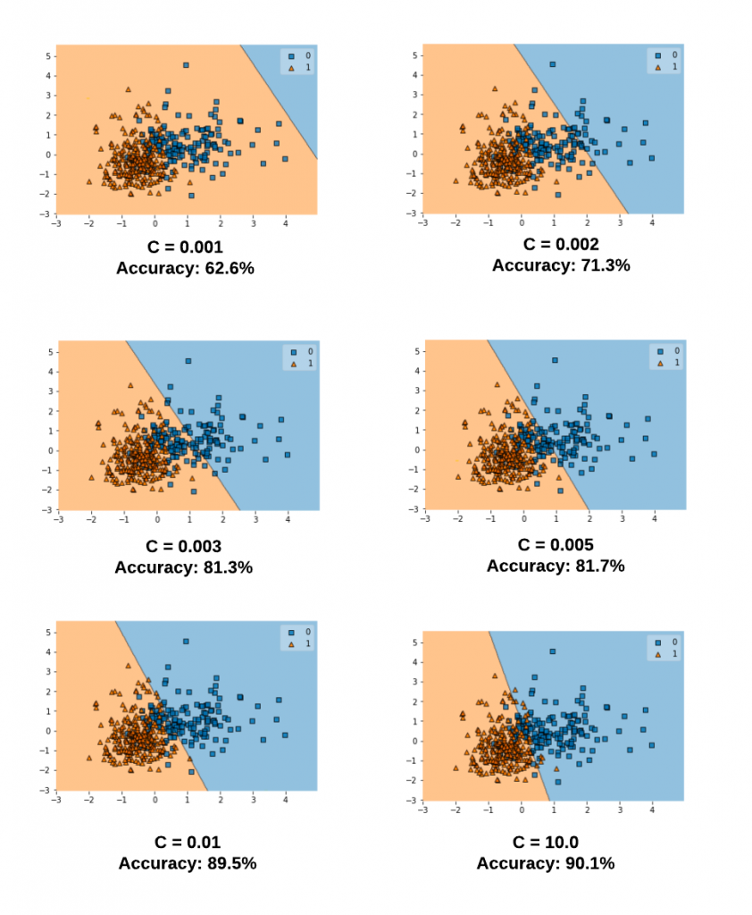
Real-world data is rarely perfectly clean. Often, classes overlap. A "hard-margin" SVM that insists on perfectly separating all points would fail in this scenario.

To handle this, we use a "soft-margin" SVM, which is controlled by the regularization parameter C. This parameter controls the trade-off between maximizing the margin and minimizing the classification error on the training set.

• Low C: The model prioritizes a wide margin, even if it means misclassifying some training points. This creates a simpler, smoother decision boundary that is less likely to overfit (higher bias).
• High C: The model prioritizes classifying all training points correctly, leading to a narrower margin and a more complex decision boundary. This can lead to overfitting (higher variance).

SVM in Practice with scikit-learn

Now, let's put all these concepts together and build an SVM classifier in Python. We will follow a structured, robust workflow that you can apply to your own projects.

Let's break down the key steps from the article you just read.

Step 1: Feature Scaling (A Critical Prerequisite)

As the article emphasizes, SVMs are not scale-invariant. The algorithm is based on calculating distances between points. If one feature (e.g., salary, 0-100,000) is on a much larger scale than another (e.g., years of experience, 0-50), the larger feature will dominate the distance calculation, and the model will perform poorly.

Rule #1 of SVMs: You must scale your features before training. StandardScaler is the most common choice.

Step 2: Using a Pipeline

The best way to chain the scaling and modeling steps is with a scikit-learn Pipeline. This ensures that the scaler is fitted only on the training data and then used to transform both the training and test data, preventing data leakage.

Step 3 & 4: Training, Tuning, and Evaluation

Here is the complete code that puts everything together. It follows the structure from the DZone article, using make_classification to create a sample dataset.

import numpy as np
import matplotlib.pyplot as plt
from sklearn.datasets import make_classification
from sklearn.model_selection import train_test_split, GridSearchCV
from sklearn.preprocessing import StandardScaler
from sklearn.svm import SVC
from sklearn.pipeline import Pipeline
from sklearn.metrics import classification_report, confusion_matrix, RocCurveDisplay

# 1. Create a synthetic dataset
X, y = make_classification(
    n_samples=1000,
    n_features=2,
    n_informative=2,
    n_redundant=0,
    random_state=42
)

# 2. Split into training and testing sets
X_train, X_test, y_train, y_test = train_test_split(X, y, test_size=0.3, random_state=42)

# 3. Create a pipeline that first scales the data, then trains the SVM
# probability=True is needed to plot the ROC curve later
svm_pipeline = Pipeline([
    ('scaler', StandardScaler()),
    ('svm', SVC(kernel='rbf', probability=True, random_state=42)) 
])

# 4. Define the grid of hyperparameters to search
# We are tuning the 'C' and 'gamma' parameters of the 'svm' step in our pipeline
param_grid = {
    'svm__C': [0.1, 1, 10, 100],
    'svm__gamma': [1, 0.1, 0.01, 0.001]
}

# 5. Use GridSearchCV to find the best hyperparameters
# We pass the entire pipeline to GridSearchCV. This is crucial!
# It ensures that for each fold of cross-validation, the scaling is learned only on that fold's training data.
grid_search = GridSearchCV(
    svm_pipeline, param_grid, cv=5, scoring='roc_auc', verbose=1, n_jobs=-1
)

print("Running GridSearchCV...")
grid_search.fit(X_train, y_train)

# 6. Get the best model and evaluate it
print(f"\nBest parameters found: {grid_search.best_params_}")
best_svm = grid_search.best_estimator_

# Make predictions on the test set
y_pred = best_svm.predict(X_test)

# Print classification report and confusion matrix
print("\n--- Classification Report (Tuned Model) ---")
print(classification_report(y_test, y_pred))

print("\n--- Confusion Matrix (Tuned Model) ---")
print(confusion_matrix(y_test, y_pred))

# Plot the ROC curve
print("\nPlotting ROC Curve...")
fig, ax = plt.subplots(figsize=(8, 6))
RocCurveDisplay.from_estimator(best_svm, X_test, y_test, ax=ax)
ax.plot([0, 1], [0, 1], color='gray', lw=2, linestyle='--', label='Random Chance')
ax.set_title('ROC Curve for Tuned SVM')
ax.legend()
plt.show()

This code is a robust template for applying SVMs. It properly handles data scaling, finds the best C and gamma through cross-validation, and provides a thorough evaluation of the final model's performance on unseen data.

Conclusion

You have now added Support Vector Machines to your machine learning toolkit. You've moved from ensemble methods to a geometric, margin-maximizing approach to classification.

Key Takeaways:

• SVMs aim to find an optimal hyperplane that creates the maximum margin between classes.
• The model's decision boundary is defined by the support vectors—the points closest to the margin.
• The kernel trick (e.g., with the RBF kernel) allows SVMs to find non-linear decision boundaries by implicitly projecting data into higher dimensions.
• The gamma parameter controls the influence of support vectors, affecting the complexity of the RBF kernel's boundary.
• The regularization parameter C controls the trade-off between a wide margin and correctly classifying training points, helping to prevent overfitting.
• Feature scaling is mandatory for SVMs, and using a Pipeline is the best practice for implementation.

Preview of the Next Module:

So far, all the algorithms we've studied—from Linear Regression to Gradient Boosting and SVMs—have been forms of supervised learning. They all require labeled data (features X and a target y). In the next module, we will venture into a new and exciting area: Unsupervised Learning, where we work with data that has no predefined labels. Our first lesson will be on Principal Component Analysis (PCA), a powerful technique for dimensionality reduction.