Building and Evaluating Random Forests

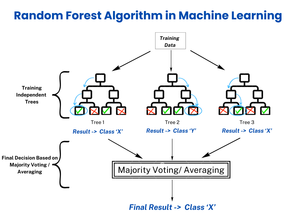
From a Single Tree to a Forest

The main problem with a single decision tree is its high variance. It can learn the training data, including its noise, too well. A Random Forest is an ensemble method designed to reduce this variance by averaging out the errors of many individual trees.

How does it ensure that the trees are different from each other? It introduces randomness in two key ways.

Let's watch a video that visualizes these two concepts: Bootstrapping and Random Feature Selection.

To summarize, a Random Forest builds multiple decision trees, where each tree is trained on:

1. A bootstrap sample of the data (randomly selected rows, with replacement).
2. With splits chosen from a random subset of features at each node.

Once the forest is trained, how does it make a prediction? For classification, it's simple democracy.

The combination of these techniques makes Random Forests one of the most reliable and widely used machine learning algorithms. Here is a helpful table comparing it to the single Decision Tree you learned about last time.

Building a Random Forest with scikit-learn

Now for the practical part. Since a Random Forest is an ensemble of decision trees, you'll find its implementation in scikit-learn's ensemble module. The workflow is identical to what you've seen before.

The following video demonstrates the entire process, from loading data to training the model and checking its performance.

Here's the essential code structure for building and training your model:

from sklearn.datasets import make_classification
from sklearn.model_selection import train_test_split
from sklearn.ensemble import RandomForestClassifier
from sklearn.metrics import accuracy_score

# 1. Generate some data
X, y = make_classification(n_samples=1000, n_features=20, n_informative=15, n_redundant=5, random_state=42)

# 2. Split data
X_train, X_test, y_train, y_test = train_test_split(X, y, test_size=0.3, random_state=42)

# 3. Create and train the Random Forest model
# The model is in the 'ensemble' module
# We start with 100 trees (n_estimators=100)
rf_clf = RandomForestClassifier(n_estimators=100, random_state=42, n_jobs=-1)
rf_clf.fit(X_train, y_train)

# 4. Make predictions and evaluate
y_pred = rf_clf.predict(X_test)
accuracy = accuracy_score(y_test, y_pred)
print(f"Accuracy: {accuracy:.4f}")

Notice the n_jobs=-1 parameter. This is a practical tip: it tells scikit-learn to use all available CPU cores to build the trees in parallel, which can significantly speed up training.

Key Hyperparameters

While a Random Forest has many hyperparameters, two are most fundamental to its structure. The others, like max_depth and min_samples_leaf, are the same as those for individual decision trees and control the complexity of each tree in the forest.

1. n_estimators: The number of trees in the forest.

   • This is the most important hyperparameter.
   • Generally, more trees increase the model's performance and stability, but the benefit diminishes after a certain point.
   • More trees also mean longer training and prediction times. The default in scikit-learn is 100, which is often a reasonable starting point.

2. max_features: The size of the random subset of features to consider at each split.

   • Lowering this value reduces the correlation between trees, which can help combat overfitting.
   • The default is 'sqrt' (the square root of the total number of features), which is a common and effective choice.

Evaluating Random Forest Performance

You can evaluate a Random Forest using the same metrics as any other classifier, like accuracy and the confusion matrix. But it also comes with some unique, built-in evaluation tricks.

Out-of-Bag (OOB) Score

Remember that each tree is trained on a bootstrap sample, which means it doesn't see all the training data. On average, about one-third of the training samples are left out for each tree. These are the Out-of-Bag (OOB) samples.

We can use these OOB samples as a built-in validation set to evaluate the model's performance without needing a separate train-test split. This is particularly useful when you have a small dataset.

To use this in scikit-learn, you simply set oob_score=True when creating your classifier. After training, you can access the score via the .oob_score_ attribute.

# Create a model with OOB scoring enabled
rf_clf_oob = RandomForestClassifier(n_estimators=100, oob_score=True, random_state=42, n_jobs=-1)

# Fit the model (only on training data)
rf_clf_oob.fit(X_train, y_train)

# Access the OOB score
print(f"OOB Score: {rf_clf_oob.oob_score_:.4f}") 
# This score is calculated using data not seen by each tree during training.

Feature Importance

Because a Random Forest uses many trees, it can provide a more robust and reliable estimate of feature importance than a single decision tree. It calculates importance by averaging the impurity decrease contributed by each feature across all trees in the forest. This is a great way to understand what features are driving your model's predictions.

Here is how you can access and plot them:

import pandas as pd
import matplotlib.pyplot as plt

# Assuming rf_clf is your trained model and X_train has feature names
importances = rf_clf.feature_importances_
feature_names = [f"feature_{i}" for i in range(X.shape[1])] # Example feature names

forest_importances = pd.Series(importances, index=feature_names)

fig, ax = plt.subplots()
forest_importances.sort_values(ascending=False).head(10).plot.bar(ax=ax)
ax.set_title("Top 10 Feature importances using MDI")
ax.set_ylabel("Mean decrease in impurity")
fig.tight_layout()
plt.show()

Conclusion

Congratulations! You've mastered another state-of-the-art classification algorithm. Random Forests are a go-to model for many data scientists because they are powerful, relatively easy to use, and less prone to overfitting than single decision trees.

Key Takeaways:

• Random Forests are an ensemble of decision trees that improve accuracy and reduce variance.
• They introduce randomness through bagging (bootstrap sampling of data) and random feature subspaces.
• Predictions are made by majority vote (for classification).
• The most important hyperparameter is n_estimators (the number of trees).
• They offer powerful built-in evaluation methods like the Out-of-Bag (OOB) score and robust feature importance measures.

Preview of the Next Lesson:

Random Forest is one type of ensemble method, where models are built independently and in parallel. But what if we built them sequentially, where each new model tries to fix the mistakes of the previous one? This is the idea behind another powerful family of algorithms called boosting. In our next lesson, we will explore Gradient Boosting, a technique that often pushes the boundaries of predictive accuracy even further.