Multiclass Logistic Regression with scikit-learn

From Binary to Multiclass: The Strategies

How can we adapt an algorithm designed for two classes (0 or 1) to handle three, ten, or even a hundred classes? There are two primary strategies for extending logistic regression to multiclass problems.

1. One-vs-Rest (OvR): Also known as One-vs-All. This strategy is quite intuitive. If you have K classes, you train K separate binary logistic regression classifiers. Each classifier is trained to distinguish one class (the "one") from all other classes combined (the "rest"). When you want to predict a new instance, you run it through all K classifiers, and the one that outputs the highest probability wins.

2. Multinomial (Softmax) Regression: Instead of training multiple independent classifiers, this approach generalizes logistic regression in a single model. It uses a function called Softmax, which is the multiclass equivalent of the sigmoid function you learned about. It computes a score for each class and then converts those scores into a probability distribution where all probabilities sum to 1.

Understanding Softmax Regression

Since you appreciate the "why" behind the algorithms, let's briefly look at how Softmax works. It's a natural extension of the concepts from our last lesson.

1. Linear Score: For each class k (out of K total classes), the model calculates a linear score, just like in binary regression: $z_k={\theta }_k^{T}x$. This gives us a vector of scores $[z_1,z_2,\dots ,z_K]$.

2. Exponentiation: The scores are then exponentiated to make them all positive: $e^{z_k}$.

3. Normalization: Finally, each exponentiated score is divided by the sum of all exponentiated scores. This step normalizes the values so they become probabilities that sum to 1. The probability of the instance belonging to class k is:
   $P(y=k|x)=\frac{e^{z_k}}{{\sum }_{j=1}^K{e}^{z_j}}$

This is the Softmax function.

To see this in action, watch the following short video from Andrew Ng's DeepLearning.AI course. It provides a clear conceptual overview and a numerical example.

Now, let's put this theory into practice.

Implementing Multiclass Logistic Regression with scikit-learn

While it's valuable to understand the mechanics, for practical applications, we use libraries like scikit-learn. They provide highly optimized, robust, and easy-to-use implementations.

We'll walk through a classic multiclass problem: recognizing handwritten digits. The following video by codebasics is an excellent guide. You'll see how to load the data, train a model, and evaluate its performance in just a few lines of code.

As you saw in the video, the core steps are:

1. Load Data: scikit-learn has convenient functions like load_digits() for datasets.
2. Split Data: train_test_split is used to create training and testing sets, which is crucial for unbiased model evaluation.
3. Instantiate and Train: You create an instance of the LogisticRegression class and call the .fit(X_train, y_train) method. scikit-learn handles all the gradient descent optimization internally!

Evaluating Multiclass Classification Performance

After training, how do we know if our model is any good? The .score() method gives us the overall accuracy, which is a good starting point. However, accuracy doesn't tell the whole story. It doesn't show us what kinds of mistakes the model is making. For that, we use a confusion matrix.

A confusion matrix for a K-class problem is a KxK table where:

• The rows represent the True Labels.
• The columns represent the Predicted Labels.
• The cell at (i, j) contains the number of instances of true class i that were predicted as class j.

Correct predictions lie on the diagonal (where i=j), while all off-diagonal cells represent errors. This helps you instantly see if the model is confusing specific classes (e.g., frequently mistaking a '3' for an '8').

Let's see how to generate and interpret one.

OvR vs. Multinomial: Which to Choose?

In scikit-learn, you can control the multiclass strategy with the multi_class parameter in LogisticRegression. The default is 'auto', which tries to pick the best strategy based on the data and the chosen solver. You can explicitly set it to 'ovr' for One-vs-Rest or 'multinomial' for Softmax regression.

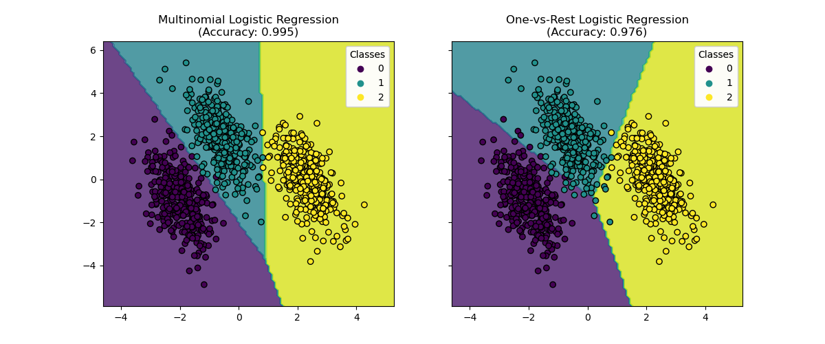
So, which one should you use? The following article provides an excellent breakdown.

Key takeaways from the reading:

• 'multinomial' (Softmax) is often more accurate, especially if classes overlap, because it models the probabilities jointly. However, it's computationally more intensive and only compatible with specific solvers (like 'lbfgs', 'newton-cg', 'saga').
• 'ovr' is faster and works with all solvers (including 'liblinear', which is great for large or sparse datasets). It's a solid baseline approach.
• Hyperparameter Tuning is crucial. Finding the optimal C (regularization strength) and solver for your specific problem can significantly boost performance. Using GridSearchCV is a systematic way to do this.

Beyond the confusion matrix, you can also use metrics like precision, recall, and F1-score for multiclass problems. scikit-learn allows you to calculate these by specifying an averaging method ('micro', 'macro', or 'weighted') to aggregate the scores from each class. The article "Logistic Regression and Evaluation Metrics" explains this well in its "Evaluation Metrics for Multiclass Classification" section, which you can refer to for more detail.

Conclusion

Congratulations! You've successfully made the leap from binary to multiclass classification. You now have the tools to tackle a much wider range of real-world problems.

Key Takeaways:

• Logistic regression can be extended to multiclass problems using the One-vs-Rest (OvR) or Multinomial (Softmax) strategies.
• scikit-learn provides a powerful LogisticRegression class that makes training and evaluating these models straightforward.
• The confusion matrix is an essential tool for understanding a classifier's performance in detail, showing not just if it made errors, but what kind of errors it made.
• Choosing the right strategy ('ovr' vs. 'multinomial') and tuning hyperparameters like solver and C are key to building high-performing models.

Preview of the Next Lesson:

So far, we've focused on logistic regression, which is a powerful linear model. It works by creating linear decision boundaries to separate classes. In the next lesson, we will explore a completely different type of classifier: the Decision Tree. This is a non-linear model that learns a set of hierarchical rules, which can capture more complex patterns in data.