Logistic Regression from Scratch

From Linear Regression to Probabilities

Let's start with a familiar concept: the linear regression equation.
$z={\theta }^{T}x={\theta }_0+{\theta }_1{x}_1+{\theta }_2{x}_2+\cdots +{\theta }_n{x}_n$
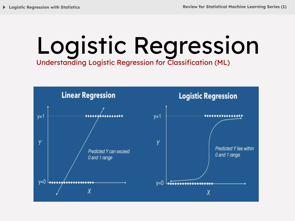
As you know, this produces a continuous output. But for binary classification, we need a prediction of either 0 or 1. How can we map the continuous output z to a binary outcome?

A naive approach might be to set a threshold: if z > 0, predict 1; otherwise, predict 0. However, this is very sensitive to outliers and doesn't give us a measure of confidence. A much better approach is to convert the output z into a probability.

This is where the Sigmoid function (also called the logistic function) comes in. It takes any real number and "squashes" it into a value between 0 and 1.

$h_{\theta }(x)=g(z)=\frac{1}{1+e^{-z}}$

The output, $h_{\theta }(x)$, can be interpreted as the probability that the label y is 1, given the input x and parameters $\theta$. For example, if $h_{\theta }(x)=0.8$, the model is 80% confident that the class is 1.

To make a final decision, we use a decision boundary. A common choice is a threshold of 0.5:

• If $h_{\theta }(x)\ge 0.5$, we predict class 1.
• If $h_{\theta }(x)<0.5$, we predict class 0.

Let's watch a video that walks through this core concept.

The Cost Function for Classification

In linear regression, we used Mean Squared Error (MSE) to measure our model's error. Why can't we use it here? If we plug our sigmoid-based hypothesis into the MSE formula, the resulting cost function is non-convex—it has many local minima. This makes it very difficult for an optimization algorithm like gradient descent to find the optimal parameters.

Instead, we need a cost function that is convex and suited for measuring the error between a predicted probability and a true binary label (0 or 1). This function is called Cross-Entropy Loss, or Log Loss.

The formula for a single training example is:
$\text{Cost}(h_{\theta }(x),y)=\{\begin{array}{ll}-\log (h_{\theta }(x))& \text{if }y=1\\ -\log (1-h_{\theta }(x))& \text{if }y=0\end{array}$

• If the true label y is 1: The cost is -\log(prediction). If our model correctly predicts a probability close to 1 (e.g., 0.99), the cost is very low. If it incorrectly predicts a probability close to 0 (e.g., 0.01), the cost is very high.
• If the true label y is 0: The cost is -\log(1 - prediction). The logic is the same but reversed.

This piecewise function can be elegantly combined into a single equation for the average cost over all m training examples:
$J(\theta )=-\frac{1}{m}{\sum }_{i=1}^m\left[y^{(i)}\log (h_{\theta }(x^{(i)}))+(1-y^{(i)})\log (1-h_{\theta }(x^{(i)}))\right]$

This is the function we want to minimize. The following video segment derives this formula starting from the principle of maximum likelihood, which provides a strong theoretical justification for its use.

Optimization with Gradient Descent

Now that we have a convex cost function $J(\theta )$, we can use gradient descent to find the parameters $\theta$ that minimize it. As you'll recall from our calculus module, this involves iteratively updating the parameters in the opposite direction of the gradient.

The update rule remains the same:
${\theta }_j:={\theta }_j-\alpha \frac{\partial }{\partial {\theta }_j}J(\theta )$
Our task is to find the partial derivative of the cross-entropy cost function with respect to each parameter ${\theta }_j$. Given your background in calculus, you'll appreciate seeing the full derivation, which uses the chain rule.

The final result for the partial derivative is remarkably simple and elegant:
$\frac{\partial }{\partial {\theta }_j}J(\theta )=\frac{1}{m}{\sum }_{i=1}^m(h_{\theta }(x^{(i)})-y^{(i)})x_j^{(i)}$
This formula calculates the average error for each data point, weighted by the corresponding feature value, to determine how to adjust each weight.

The next video segment will walk you through this derivation step-by-step.

Implementing Logistic Regression from Scratch

Now for the most exciting part: translating this theory into working Python code. We will build a LogisticRegression class from scratch using NumPy. This will solidify your understanding of every component.

Our implementation will consist of a few key parts:

1. A _sigmoid function: To compute the sigmoid activation.
2. A fit method: To train the model using gradient descent. This method will initialize the weights and iteratively update them by calculating the gradient.
3. A predict method: To make predictions on new data using the learned weights and a decision threshold.

The final segments of the video we've been watching provide a complete, line-by-line walkthrough of this implementation. It uses vectorized NumPy operations, which is highly efficient and builds upon what you learned in the NumPy module.

Here's a summary of the key functions you'll be building, based on the video's approach. This structure is a great template for your own implementation.

import numpy as np

class LogisticRegression:
    def __init__(self, learning_rate=0.01, n_iterations=1000):
        self.learning_rate = learning_rate
        self.n_iterations = n_iterations
        self.weights = None
        self.bias = None

    def _sigmoid(self, z):
        return 1 / (1 + np.exp(-z))

    def fit(self, X, y):
        n_samples, n_features = X.shape
        
        # Initialize parameters
        self.weights = np.zeros(n_features)
        self.bias = 0

        # Gradient Descent
        for _ in range(self.n_iterations):
            # Calculate linear model and apply sigmoid
            linear_model = np.dot(X, self.weights) + self.bias
            y_predicted = self._sigmoid(linear_model)

            # Calculate gradients
            dw = (1 / n_samples) * np.dot(X.T, (y_predicted - y))
            db = (1 / n_samples) * np.sum(y_predicted - y)

            # Update parameters
            self.weights -= self.learning_rate * dw
            self.bias -= self.learning_rate * db
    
    def predict(self, X):
        linear_model = np.dot(X, self.weights) + self.bias
        y_predicted_probs = self._sigmoid(linear_model)
        
        # Apply decision boundary
        y_predicted_class = [1 if i > 0.5 else 0 for i in y_predicted_probs]
        return np.array(y_predicted_class)

Note: The video implements the bias term slightly differently by adding a column of ones to X. The separate bias term shown here is an alternative common practice. Both are mathematically equivalent and good to know.

Conclusion

Fantastic work! You have successfully built a fundamental machine learning algorithm from the ground up. You've gone from the theoretical underpinnings to a practical, working implementation.

Key Takeaways:

• Logistic Regression is a classification algorithm that models the probability of a binary outcome.
• It combines a linear equation with the sigmoid function to produce a probability between 0 and 1.
• The appropriate cost function is Cross-Entropy Loss, which is convex and penalizes confident, incorrect predictions.
• Gradient descent is used to minimize this cost function by iteratively updating the model's weights and bias based on the calculated gradients.

By implementing this yourself, you've gained an intuition that is impossible to get just from using a library.

Preview of the Next Lesson:

Now that you understand the mechanics of logistic regression, we'll see how to use the highly-optimized implementation available in scikit-learn. We will also explore how to extend the model from binary to multiclass classification, allowing you to tackle problems with more than two categories.