Hello! Welcome to the final lesson in our module on regression.
In our last session, we focused on interpreting the coefficients of a trained regression model. You learned how a coefficient represents the relationship between a single feature and the target, allowing you to understand what your model has learned.
Today, we shift our focus to assessing how well the model performs. While you've already calculated basic metrics, this lesson will provide a deeper understanding of the key tools for model evaluation. We will explore quantitative metrics like Mean Squared Error (MSE) and R-squared, and then move to a powerful qualitative technique: residual analysis. By the end of this lesson, you will be able to confidently assess the fit and predictive power of your regression models.
The Foundation of Error: Residuals
Before we can evaluate a model, we must first understand what an "error" is in the context of regression. The fundamental unit of error is the residual.
A residual is simply the difference between the actual value and the predicted value for a single data point.
A positive residual means the model's prediction was too low, while a negative residual means the prediction was too high. Our goal in regression is to make these residuals as small as possible, on average, across all data points.
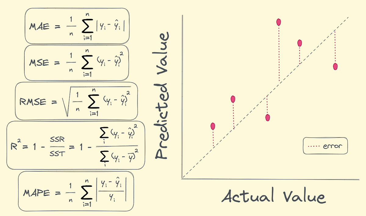
Metric 1: Mean Squared Error (MSE) and RMSE
We need a way to aggregate all the individual residuals into a single number that summarizes the model's overall error. One of the most common ways to do this is with Mean Squared Error (MSE).
The formula for MSE is:
In simple terms, for each data point, we:
- Calculate the residual.
- Square it.
- Average all these squared residuals.
Squaring the residuals is important for two reasons:
- It ensures that positive and negative residuals don't cancel each other out.
- It penalizes larger errors more heavily than smaller ones.
A related and often more useful metric is the Root Mean Squared Error (RMSE), which is just the square root of the MSE. The advantage of RMSE is that its value is in the same units as your target variable, making it more interpretable. For example, if you're predicting house prices in dollars, an RMSE of 5000 means your model's predictions are, on average, off by about $5,000. For both MSE and RMSE, a lower value is better.
Let's get a formal overview of these metrics and how to implement them.
Sklearn Linear Regression: A Complete Guide
The DataCamp article 'Sklearn Linear Regression: A Complete Guide' offers a clear, concise explanation of MSE and RMSE, complete with the scikit-learn code to calculate them.
Please read the section titled 'Evaluating model performance'. Focus on the definitions and formulas for Mean Squared Error (MSE) and Root Mean Squared Error (RMSE). Note the interpretation that lower values indicate a better model fit.
Metric 2: R-squared (The Coefficient of Determination)
MSE and RMSE are great for understanding the absolute error of a model, but they don't tell you if your model is "good" in a relative sense. An RMSE of $5,000 might be excellent for a model predicting million-dollar homes but terrible for a model predicting the price of a t-shirt.
This is where R-squared (R²) comes in. It provides a relative measure of fit, typically ranging from 0 to 1. R-squared tells you the proportion of the variance in the target variable that is explained by your model's features.
- An R² of 0.85 means that your model explains 85% of the variability in the target data.
- An R² of 0 means your model is no better than a naive model that just predicts the average value of the target every time.
- A higher R² is generally better.
To develop a strong intuition for this crucial metric, the following video is one of the best explanations available.
R-squared, Clearly Explained!!!
To really understand what R-squared represents, there's no better source than StatQuest. This video will walk you through the concept intuitively, explaining it as the percentage of variation that your model successfully explains.
Watch from 01:30 to 08:08. Pay close attention to the core concepts of 'variation around the mean' versus 'variation around the regression line', and see how they are combined to calculate R-squared.
Given your programming background, seeing how R-squared is built from the ground up in code can solidify this understanding. The following resource does exactly that.
Regression Analysis with Scikit-Learn (part 1 - Linear)
The 'Programming Historian' article provides a Python function that calculates R-squared from scratch. This is a great way to connect the theory from the video directly to a practical implementation.
Read the section 'Step 8: Evaluating Performance'. Study the r_square_scratch function to see how the R-squared formula is implemented using basic Python operations. Compare the steps in the code to the logic explained in the StatQuest video.
Diagnostic Tool: Residual Analysis
Single-number metrics like R² and MSE are useful summaries, but they can hide underlying problems with your model. Residual analysis is the practice of plotting your model's residuals to visually diagnose its performance and check if the assumptions of linear regression are met.
Two plots are fundamental here:
1. Residuals vs. Predicted Values Plot
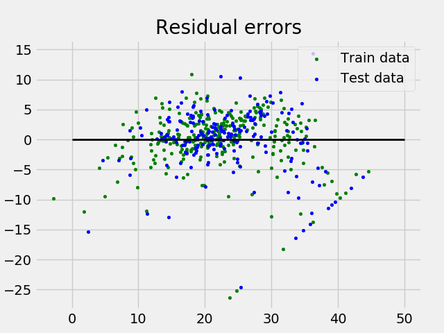
This is the most important diagnostic plot. You plot the predicted values () on the x-axis and the corresponding residuals () on the y-axis.
- What you want to see: A random, "boring" scatter of points centered around the y=0 line. There should be no discernible pattern. This indicates that the model's errors are random, which is good.
- What you don't want to see (Red Flags):
- A U-shape or curved pattern: This suggests the relationship between your features and target is not linear, and a simple linear model is not appropriate.
- A funnel shape (heteroscedasticity): The plot is wider on one side than the other. This means the model's error is not constant; it makes better predictions for some ranges of values than others.
2. Histogram of Residuals
This plot shows the distribution of your model's errors. One of the assumptions of linear regression is that the errors are normally distributed.
- What you want to see: A roughly symmetric, bell-shaped curve centered at 0. This suggests the assumption of normally distributed errors is met.
Let's see how to generate and interpret these plots in Python.
Linear Regression And Residuals - Pandas For Machine Learning 28
This segment from Codemy.com provides a quick, practical demonstration of how to create and analyze a residual plot in Python.
Watch from 15:03 to 17:28. Focus on the explanation of the residual plot. Listen for the key takeaway: a good residual plot should show a random scatter of points around zero with no discernible trend.
For a clear, written guide with another code example, the DataCamp article is a great reference.
Sklearn Linear Regression: A Complete Guide
The DataCamp article also provides an excellent summary and code for creating these diagnostic plots using seaborn.
Navigate to the section 'Summarizing model results' and review the code and explanations for the 'Residuals Distribution' (a histogram) and 'Regression Fit (Actual vs Predicted)' plots.
Test your understanding!
You have trained three different linear regression models to predict student test scores (0-100). You get the following results:
- Model A: R² = 0.85, RMSE = 8. A plot of its residuals vs. predicted values shows a random scatter of points around y=0.
- Model B: R² = 0.92, RMSE = 5. A plot of its residuals vs. predicted values shows a clear U-shape.
- Model C: R² = 0.50, RMSE = 20. A plot of its residuals vs. predicted values shows a random scatter of points around y=0.
Which model would you choose and why? What is wrong with the other models?
Show answer
Model A is the best choice.
- Why Model A is best: It has a high R² (explains 85% of the variance) and a reasonably low RMSE. Crucially, its residual plot is random, indicating that the assumptions of the linear model are met. The model is a good and reliable fit.
- What's wrong with Model B: Despite having the best R² and RMSE, the U-shaped residual plot is a major red flag. It indicates that the underlying relationship in the data is non-linear. A linear model is not appropriate here, and its predictions would be systematically biased. You cannot trust this model.
- What's wrong with Model C: While its residual plot looks good (meaning a linear model is appropriate), its performance metrics (low R² and high RMSE) are poor. It's a valid model, but not a very useful one.
This highlights a key lesson: metrics alone are not enough. You must also perform residual analysis to validate that your model is appropriate for the data.
Conclusion
Congratulations on completing this deep dive into regression model evaluation! You are now equipped with a powerful toolkit to not only measure but also diagnose the performance of your models.
Key Takeaways:
- MSE and RMSE measure the average prediction error of your model in absolute terms. Lower is better.
- R-squared (R²) measures the proportion of variance in the target that your model explains, providing a relative measure of fit. Higher is better.
- Residual Analysis is a critical diagnostic step. By plotting residuals, you can visually check if the assumptions of your linear model are met and identify issues like non-linearity or non-constant error variance.
Preview of the Next Lesson:
This lesson concludes our module on Supervised Learning for Regression. You can now build, interpret, and thoroughly evaluate models that predict continuous values.
In the next module, we will pivot to an entirely new and equally important domain: Classification. Our goal will no longer be to predict a number, but to predict a discrete category (e.g., 'spam' or 'not spam', 'cat' or 'dog'). We will begin by implementing the foundational classification algorithm, Logistic Regression, from scratch.