Interpreting Regression Coefficients

The Linear Regression Equation and its Coefficients

Let's quickly revisit the equation for multiple linear regression:

When you train a model in scikit-learn, it solves for the optimal values of these parameters:

• ${\beta }_0$ is the intercept, which you can access via model.intercept_.
• ${\beta }_1,{\beta }_2,\dots ,{\beta }_p$ are the coefficients for each feature $x_1,x_2,\dots ,x_p$, which you can access as an array via model.coef_.

The following video provides a great refresher on how these mathematical terms map directly to the attributes of a trained scikit-learn model.

Now that we know where to find these coefficients, let's learn how to interpret what they mean.

Interpreting Coefficients of Numerical Features

The interpretation of a coefficient for a numerical feature is the most straightforward.

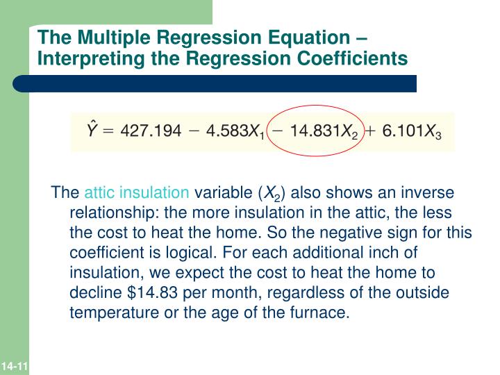
A coefficient represents the expected change in the target variable for a one-unit increase in the corresponding feature, assuming all other features are held constant.

This "holding all other features constant" part is crucial. We are trying to isolate the impact of a single feature.

To see this in action with code, we'll use an excellent article from Machine Learning Mastery that uses the Ames Housing dataset to predict SalePrice.

As the article explains, a coefficient of 110.52 for GrLivArea means that, on average, for each additional square foot of living area, the house's sale price is predicted to increase by $110.52, all else being equal.

The book "Interpretable Machine Learning" provides a useful template for this interpretation.

Interpreting Coefficients of Categorical Features

Interpreting categorical features is a bit more nuanced because they are typically transformed using one-hot encoding first (as you learned in Module 5).

When you one-hot encode a feature, you create new binary (0/1) columns for each category. To avoid multicollinearity, one category is usually dropped and becomes the reference category.

• The model's intercept (${\beta }_0$) now represents the average prediction for this reference category (when all numerical features are 0).
• The coefficient for another category represents the difference in the predicted target between that category and the reference category.

Let's return to the Machine Learning Mastery article, which has a fantastic explanation of this process.

From the article, the model's intercept is about $96,827, which is the average price in the reference neighborhood, "MeadowV". The coefficient for "BrkSide" is $29,235. This means a house in "BrkSide" is predicted to cost, on average, $29,235 more than a similar house in "MeadowV".

Important Considerations and Caveats

While coefficient interpretation is powerful, there are two critical points to remember.

1. Correlation and Context Matter

A feature's coefficient can change depending on what other features are in the model. This happens because features are often correlated. For example, the value of an extra square foot of living area might be different in an expensive neighborhood compared to a cheaper one.

The Machine Learning Mastery article demonstrates this beautifully.

This shows that a coefficient's value is not an absolute truth but is always interpreted in the context of the other features in the model.

2. Coefficient Magnitude is Not Feature Importance (Without Scaling)

It is tempting to look at the coefficients and assume that the feature with the largest coefficient is the most "important." This is often incorrect.

The scale of the feature affects the scale of its coefficient. Imagine a feature distance_in_km with a coefficient of 10. If you change the feature to distance_in_meters, its values will be 1000 times larger, and its new coefficient will become 1000 times smaller (0.01), even though the feature's underlying importance is the same.

To make coefficients more comparable for gauging importance, you should scale your numerical features (e.g., using StandardScaler, as we've done before) before training the model. After scaling, features are on a similar scale, and their coefficient magnitudes give a better (though still not perfect) sense of their relative impact.

Conclusion

Great job today! You've moved beyond just evaluating a model's score to understanding what the model has actually learned. This is the key to extracting real-world value and insights from your machine learning work.

Key Takeaways:

• A numerical feature's coefficient is the change in the target for a one-unit increase in that feature, holding others constant.
• A categorical feature's coefficient is the difference in the target compared to the reference category, holding others constant.
• The intercept is the baseline prediction when all numerical features are zero and all categorical features are at their reference category.
• The interpretation of any single coefficient is always conditional on the other features included in the model.
• You cannot compare raw coefficient magnitudes to judge feature importance unless the features have been scaled.

Preview of the Next Lesson:

In the last lesson, we calculated R² and MSE to get a single number representing model performance. In the next lesson, Assess regression model fit using R-squared, MSE, and residual analysis, we will dive deeper into model assessment. We'll focus particularly on residual analysis—analyzing the errors of our model. This is a powerful diagnostic tool that can tell us if the assumptions of linear regression are being met and help us identify where our model is going wrong.