Hello! Welcome to the final lesson on specific clustering algorithms in our Unsupervised Learning module.
In our previous lessons, we explored K-means, which partitions data into a pre-defined number of spherical clusters, and hierarchical clustering, which builds a tree of nested clusters. A common feature of both is that they assign every single data point to a cluster. This can be a limitation when dealing with real-world data that contains noise or clusters of irregular shapes.
Today, we'll address these challenges with a powerful, density-based algorithm: DBSCAN (Density-Based Spatial Clustering of Applications with Noise). Your learning goal is to use DBSCAN for density-based clustering. We'll cover the intuition behind how it works, its key parameters, and how to implement it using scikit-learn. DBSCAN operates on a simple but powerful idea: a cluster is a dense region of data points, separated from other clusters by regions of lower density.
To see why this is so useful, look at the image below. It compares the performance of DBSCAN (top row) with K-means (bottom row) on several datasets.
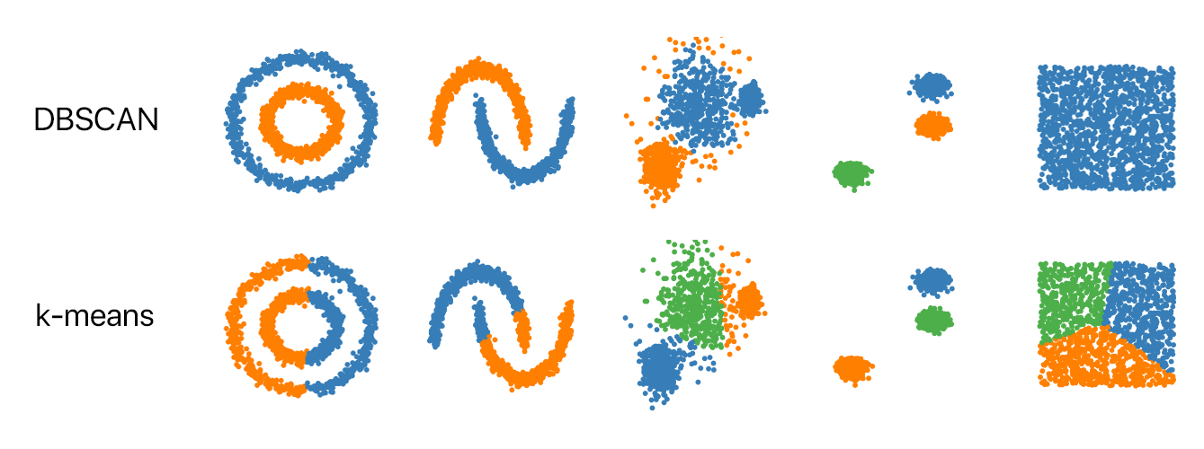
Notice how DBSCAN correctly identifies the natural structure of the data and flags outliers, while K-means makes assumptions about the cluster shape that don't always hold true.
1. The Core Concepts of DBSCAN
DBSCAN's logic is designed to mimic how we might identify clusters by eye: we look for crowded areas. To formalize this, the algorithm relies on two key parameters:
- Epsilon (): This is a distance value (a radius) that defines the "neighborhood" around a data point.
- Minimum Points (
min_samples): This is the minimum number of data points (including the point itself) that must be within a point's -neighborhood for it to be considered part of a dense region.
Based on these two parameters, DBSCAN classifies every point in the dataset into one of three types:
- Core Point: A point that has at least
min_sampleswithin its -radius. These points are in the interior of a cluster. - Border Point (or Non-Core Point): A point that is within the -radius of a core point but does not have
min_samplesin its own neighborhood. These points are on the edges of a cluster. - Noise Point (or Outlier): A point that is neither a core point nor a border point. It's isolated in a low-density region.
To get a clear, visual understanding of these concepts, the following video from StatQuest is an excellent resource.
Clustering with DBSCAN, Clearly Explained!!!
The video 'Clustering with DBSCAN, Clearly Explained!!!' provides a fantastic introduction to the motivation and core concepts of the algorithm.
Watch from the beginning to 5:08. This segment explains why we need DBSCAN, defines the ε (epsilon) radius and minimum points, and shows how these are used to classify points as core or non-core.
2. The DBSCAN Algorithm in Action
Now that you understand the different types of points, let's see how DBSCAN uses them to build clusters. The algorithm works as follows:
- It starts with an arbitrary, unvisited data point.
- It checks if the point is a core point.
- If it's not a core point, it's temporarily labeled as noise and the algorithm moves to another unvisited point.
- If it is a core point, a new cluster is created.
- The algorithm then finds all points that are "reachable" from this core point. This includes other core points in its neighborhood (which are added to a list to be visited) and any border points.
- This process continues, expanding the cluster like a chain reaction, until no more points can be added.
- Once the cluster is complete, the algorithm moves to the next unvisited point and repeats the process.
Any points that are never added to a cluster are considered noise.
The next part of the StatQuest video you started provides a great animation of this cluster-growing process.
Clustering with DBSCAN, Clearly Explained!!!
Let's continue with the StatQuest video to see how DBSCAN iteratively builds clusters.
Watch from 5:08 to 8:10. This part demonstrates the step-by-step process of forming a cluster by starting with a core point and expanding to its neighbors.
Test your understanding!
Imagine you have a set of points and you set min_samples = 4 and cm. You are analyzing a specific point, P.
Phas 5 other points within a 1 cm radius. What type of point isP?- Another point,
Q, has only 2 other points within its 1 cm radius. However, one of those neighbors is the core pointP. What type of point isQ? - A third point,
R, has 1 other point within its 1 cm radius, but neitherRnor its neighbor is within 1 cm of any core point. What type of point isR?
Show answer
Phas 5 neighbors, which is greater than or equal tomin_samples - 1 = 3. IncludingPitself, there are 6 points in its neighborhood.Pis a core point.Qdoes not have enough neighbors to be a core point itself. However, because it is within the -neighborhood of a core point (P), it is classified as a border point.Rdoes not meet the criteria for a core point and is not in the neighborhood of any core point. Therefore, it is a noise point (outlier).
3. Implementing DBSCAN in Python
Implementing DBSCAN is straightforward with scikit-learn's DBSCAN class from the sklearn.cluster module.
from sklearn.cluster import DBSCAN
import numpy as np

# Sample data
X = np.array([[1, 2], [2, 2], [2, 3],
              [8, 7], [8, 8], [25, 80]])

# Instantiate DBSCAN
# eps: The maximum distance between two samples for one to be considered as in the neighborhood of the other.
# min_samples: The number of samples in a neighborhood for a point to be considered as a core point.
dbscan = DBSCAN(eps=3, min_samples=2)

# Fit the model
dbscan.fit(X)

# Get the cluster labels
labels = dbscan.labels_

print(labels)
# Expected output: [ 0  0  0  1  1 -1]
The most important thing to note in the output is the -1. Scikit-learn uses -1 to label all points that DBSCAN has identified as noise. This is a powerful feature that distinguishes it from K-means and hierarchical clustering.
A Practical Challenge: Choosing eps
While min_samples is often set based on domain knowledge (e.g., a cluster should have at least 5 points), choosing the right eps can be tricky.
- If
epsis too small, most points will be classified as noise. - If
epsis too large, clusters will merge together.
A common heuristic to guide your choice of eps involves calculating the distance to the k-nearest neighbors for all points, where k corresponds to your min_samples value. You then plot these distances in sorted order and look for the "knee" or "elbow" in the plot. This point of maximum curvature represents a threshold where distances start increasing sharply, suggesting it's a reasonable value for eps.
The following resource explains this technique and provides a Python function to help visualize it.
Clustering with Scikit-Learn in Python
The article 'Clustering with Scikit-Learn in Python' from Programming Historian describes a practical method for determining an optimal eps value.
Please read the two short sections under the heading 'How Does DBSCAN Work?': the un-titled paragraph explaining the 'eps' selection method, and the code block for the findOptimalEps function. This provides a valuable, practical technique.
A Complete Code Example
Now, let's look at a full implementation. The following article walks through generating sample data, running DBSCAN, and visualizing the results. It's a great reference for putting all the pieces together.
performing-dbscan-clustering-with-python-and-scikit-learn. ...
The article 'Performing DBSCAN-based clustering with Python and Scikit-learn' provides a clear, complete code example.
Focus on the section 'Performing DBSCAN-based clustering with Scikit-learn'. Read through the Python code blocks to understand the entire workflow: importing libraries, generating data, initializing and fitting DBSCAN, and plotting the final clustered data. Pay close attention to how the cluster labels are used for coloring the plot.
The article also demonstrates a useful application: using DBSCAN for noise removal. Since noise points are conveniently labeled as -1, you can easily filter them out of your dataset before further analysis or modeling.
4. Advantages and Disadvantages of DBSCAN
Like any algorithm, DBSCAN has its strengths and weaknesses.
Advantages:
- Does not require you to specify the number of clusters beforehand.
- Can find arbitrarily shaped clusters.
- Is robust to outliers and has a built-in mechanism for identifying them.
Disadvantages:
- May not perform well with clusters of varying densities. It uses a single global
epsvalue, which might not be appropriate for all clusters. - Can struggle with high-dimensional data due to the "curse of dimensionality," where distance measures become less meaningful.
- Performance is sensitive to the choice of
epsandmin_samples.
Conclusion
You have now added a powerful and fundamentally different clustering algorithm to your toolkit. By focusing on density, DBSCAN overcomes some of the major limitations of partitioning and hierarchical methods.
Key Takeaways:
- DBSCAN is a density-based algorithm that groups together points that are closely packed, marking points in low-density regions as noise.
- It is defined by two parameters: (epsilon), the neighborhood radius, and
min_samples, the minimum number of points required to form a dense region. - It classifies points as core, border, or noise.
- In scikit-learn, noise points are assigned the label -1.
- DBSCAN excels at finding non-spherical clusters and is naturally robust to outliers.
Preview of the Next Lesson:
We have now learned three different clustering algorithms: K-means, Hierarchical Clustering, and DBSCAN. But how do we know if the clusters they produce are any good? In our next and final lesson of this module, we will explore methods for evaluating clustering quality, using metrics like the Silhouette Score to quantitatively assess how well-defined our clusters are.