Hierarchical Clustering and Dendrogram Analysis

1. The Concept of Hierarchical Clustering

Hierarchical clustering creates a tree-like structure of nested clusters. There are two main approaches:

1. Agglomerative (Bottom-Up): This is the more common method. It starts by treating each data point as its own cluster. Then, it iteratively merges the two closest clusters until only one cluster (containing all the data points) remains.
2. Divisive (Top-Down): This method works in the opposite direction. It starts with all data points in a single cluster and recursively splits the cluster into smaller pieces until each data point is its own cluster.

We will focus on the agglomerative approach, as it's more widely used and easier to understand.

To see this bottom-up process in action, let's watch a segment from StatQuest. It provides a clear, step-by-step walkthrough of how the algorithm identifies the most similar data points and merges them into clusters.

As you saw, the algorithm builds a hierarchy of clusters based on similarity. The output of this process is perfectly captured by a diagram called a dendrogram.

2. Understanding and Analyzing Dendrograms

A dendrogram is the primary tool for visualizing and interpreting the results of hierarchical clustering. It's a tree diagram that shows the order and similarity at which clusters were merged.

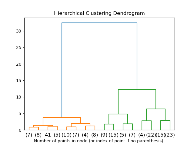
The key to reading a dendrogram is understanding the height of the branches:

• Lower branches represent merges between very similar points or clusters.
• Higher branches represent merges between less similar clusters. The longest vertical lines often represent the final merges between major, distinct groups in the data.

This article provides a concise guide on how to interpret these diagrams.

3. Key Parameters: Distance and Linkage

The agglomerative algorithm repeatedly asks, "Which two clusters are closest?" To answer this, it needs two things:

1. Distance Metric: A way to measure the distance between two individual data points. Common choices you've seen before include:

   • Euclidean distance: The straight-line distance (L2 norm).
   • Manhattan distance: The sum of absolute differences (L1 norm).

2. Linkage Criterion: A rule for measuring the distance between two clusters (which might contain multiple points). This is a new concept. The choice of linkage criterion significantly affects the shape of the final clusters. Common methods include:

   • Single Linkage: The distance between the two closest points in the respective clusters. It can produce long, "chained" clusters.
   • Complete Linkage: The distance between the two farthest points. It tends to produce compact, spherical clusters.
   • Average Linkage: The average distance between every point in one cluster and every point in the other. It's a balance between single and complete linkage.
   • Ward's Method: This is a popular default. It merges the two clusters that result in the minimum increase in the total within-cluster variance. It also tends to produce compact, evenly sized clusters.

The StatQuest video you watched earlier has excellent explanations for these concepts.

4. Implementing Hierarchical Clustering in Python

Now let's put theory into practice. In Python, the scipy.cluster.hierarchy module is the go-to tool for hierarchical clustering, especially because of its excellent functions for creating dendrograms.

The process involves two main steps:

1. Generate the linkage matrix: Using the linkage() function, we perform the hierarchical clustering. This function takes our data and the chosen method (linkage criterion, e.g., 'ward') and metric (distance metric, e.g., 'euclidean'). It returns a matrix that encodes the history of all the cluster merges.
2. Plot the dendrogram: Using the dendrogram() function, we pass the linkage matrix to generate the visual tree diagram.

The following article provides a complete, step-by-step code example.

Here's a summary of the core code from that walkthrough:

import numpy as np
from scipy.cluster.hierarchy import linkage, dendrogram
from sklearn.preprocessing import StandardScaler
import matplotlib.pyplot as plt

# 1. Sample data and scaling (scaling is crucial for distance-based algorithms!)
data = np.array([[1, 2], [2, 3], [5, 8], [8, 8], [1, 0], [0, 1]])
scaler = StandardScaler()
data_scaled = scaler.fit_transform(data)

# 2. Generate the linkage matrix using Ward's method
linkage_matrix = linkage(data_scaled, method='ward')

# 3. Plot the dendrogram
plt.figure(figsize=(10, 7))
dendrogram(linkage_matrix)
plt.title('Hierarchical Clustering Dendrogram')
plt.xlabel('Data Point Index')
plt.ylabel('Distance')
plt.show()

5. From Dendrogram to Clusters

The dendrogram shows the full hierarchy, but often we want a flat set of clusters, just like with K-means. We can achieve this by "cutting" the dendrogram at a certain height. All the clusters that exist below the cut-off line become our final clusters.

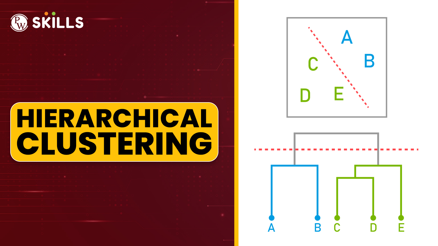
You can decide where to cut by looking for the largest vertical distance that doesn't intersect any extended horizontal lines of the dendrogram. This long vertical line suggests that two very dissimilar groups were merged, so cutting there is a reasonable choice.

Once you've decided on the number of clusters, you can use SciPy's fcluster() function to get the cluster labels for each data point.

The DataCamp article you just reviewed shows exactly how to do this. Re-examine the subsection titled "Creating clusters" within the "Implementing Hierarchical Clustering in Python" section (LINK). It uses fcluster() with the criterion='maxclust' to extract a specific number of clusters.

from scipy.cluster.hierarchy import fcluster

# Choose the number of clusters (e.g., 2, based on the dendrogram)
num_clusters = 2

# Get cluster labels by cutting the dendrogram
clusters = fcluster(linkage_matrix, t=num_clusters, criterion='maxclust')

# You can now use these 'clusters' labels for analysis or visualization
print("Cluster assignments:", clusters)
# Output might be: [2 2 1 1 2 2]

A final, important point: while dendrograms are an excellent tool for exploring potential cluster numbers, be cautious about treating them as a definitive guide for the "correct" number of clusters. As the Displayr article (LINK) notes in its "Dendrograms don’t determine cluster number" section, the visualization can sometimes suggest structure that isn't strongly supported by the data. It's best used as an exploratory tool combined with your domain knowledge.

Conclusion

Congratulations! You have now learned about a fundamentally different approach to clustering. Hierarchical clustering provides a rich, multi-level view of your data's structure, offering more flexibility than K-means.

Key Takeaways:

• Hierarchical Clustering builds a nested tree of clusters, most commonly using an agglomerative (bottom-up) approach.
• A dendrogram is a tree diagram that visualizes this hierarchy. The vertical axis represents the distance at which clusters were merged.
• The algorithm's behavior is controlled by the distance metric (e.g., Euclidean) and the linkage criterion (e.g., Ward's, complete, single).
• You can obtain a flat set of clusters by "cutting" the dendrogram at a chosen height or by specifying a desired number of clusters.
• In Python, scipy.cluster.hierarchy provides the linkage(), dendrogram(), and fcluster() functions to perform these steps.

Preview of the Next Lesson:

Both K-means and hierarchical clustering assign every single point to a cluster. But what if some data points don't naturally belong to any group? And what if clusters have irregular shapes, rather than being spherical? In our next lesson, we will explore DBSCAN, a density-based clustering algorithm that excels at finding arbitrarily shaped clusters and identifying outliers or "noise" points.