PCA for Dimensionality Reduction

The Challenge of High-Dimensionality

Imagine trying to understand a dataset with dozens or even hundreds of features. It's impossible for us to visualize data in more than three dimensions. This "Curse of Dimensionality" also poses challenges for machine learning algorithms:

• Slower Training: More features mean more computations, leading to longer training times.
• Overfitting: With many features, models might learn noise and spurious correlations specific to the training data, failing to generalize to new data.
• Redundancy: Many features might be correlated and essentially measure the same underlying property, adding complexity without adding new information.

To see why dimensionality reduction is so valuable, let's watch a short introductory video.

PCA is a feature extraction technique. Instead of just selecting a subset of the original features, it constructs a new, smaller set of features, called principal components, that are combinations of the old features.

The Core Idea: Maximizing Variance

So, how does PCA decide which new features to create? The main idea is to find the directions in the data where the variance is highest. Variance is a measure of spread; a direction with high variance is one along which the data points are most spread out, and therefore contains the most information.

PCA finds a new set of coordinates (or axes) for the data.

1. The First Principal Component (PC1) is the axis that captures the largest amount of variance in the data.
2. The Second Principal Component (PC2) is the axis, orthogonal (at a 90-degree angle) to PC1, that captures the second-largest amount of variance.
3. This continues for subsequent components, with each new component being orthogonal to all previous ones and capturing the maximum remaining variance.

This visual explanation will help solidify the concept of finding these new axes.

The Mathematics Behind PCA

Your background in computer science and mathematics will be very helpful here. The "magic" of finding these directions of maximum variance lies in linear algebra, specifically with eigenvectors and eigenvalues.

Without getting lost in the full derivation, here is the crucial insight:

The principal components of a dataset are the eigenvectors of its covariance matrix. The corresponding eigenvalue for each eigenvector tells us the amount of variance captured by that principal component.

Therefore, the first principal component is simply the eigenvector associated with the largest eigenvalue. The second principal component is the eigenvector with the second-largest eigenvalue, and so on.

Let's continue the video to see this connection explained.

This image provides a great summary of the entire process, from the initial data to the final reduced-dimension representation.

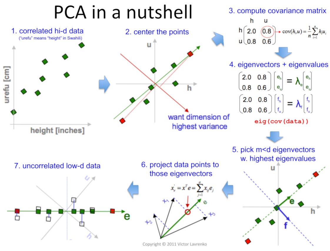
Implementing PCA with Scikit-Learn

Now that we understand the "why" and the core mathematical idea, let's focus on the "how". Fortunately, you don't need to compute covariance matrices and eigenvectors by hand. Scikit-learn provides a straightforward implementation.

The following practical guide will walk you through the entire process.

Let's consolidate the key steps from that article into a single, executable code block.

Step 1: Standardize the Data

PCA is sensitive to the scale of the features. If one feature has a much larger range than others (e.g., area in square feet vs. number of rooms), it will dominate the analysis. Therefore, it is crucial to scale your data before applying PCA. The StandardScaler is commonly used for this, which transforms each feature to have a mean of 0 and a standard deviation of 1.

Step 2: Apply PCA

We use the PCA class from sklearn.decomposition. The most important parameter is n_components, which tells scikit-learn how many dimensions to reduce the data to. You can set it in two ways:

• An integer (e.g., n_components=2): This explicitly tells PCA to return the top 2 principal components. This is useful when you know you want to visualize the data in 2D.
• A float between 0 and 1 (e.g., n_components=0.95): This tells PCA to automatically select the number of components required to capture a certain percentage (e.g., 95%) of the total variance in the data. This is the most common and recommended approach when your goal is just dimensionality reduction for a machine learning model.

Step 3: Analyze and Visualize

After fitting PCA, you can inspect the explained_variance_ratio_ attribute to see the percentage of variance captured by each component. You then use the .transform() method to project your original data onto the new principal component axes.

Here is the complete code for performing PCA on the breast cancer dataset:

import numpy as np
import pandas as pd
import matplotlib.pyplot as plt
from sklearn.datasets import load_breast_cancer
from sklearn.preprocessing import StandardScaler
from sklearn.decomposition import PCA

# --- 1. Load Data ---
data = load_breast_cancer()
X = data.data
y = data.target
target_names = data.target_names

# --- 2. Standardize the Data ---
# This is a crucial step for PCA
scaler = StandardScaler()
X_scaled = scaler.fit_transform(X)
print(f"Original shape: {X_scaled.shape}") # (569 samples, 30 features)

# --- 3. Apply PCA ---
# We want to reduce to 2 dimensions for visualization
pca = PCA(n_components=2)
principal_components = pca.fit_transform(X_scaled)

# Create a DataFrame with the principal components
pc_df = pd.DataFrame(data=principal_components, columns=['PC1', 'PC2'])
pc_df['target'] = y

# --- 4. Analyze Explained Variance ---
explained_variance = pca.explained_variance_ratio_
print(f"\nExplained variance by PC1: {explained_variance[0]:.2%}")
print(f"Explained variance by PC2: {explained_variance[1]:.2%}")
print(f"Total variance captured by 2 components: {np.sum(explained_variance):.2%}")

# --- 5. Visualize the Results ---
plt.figure(figsize=(10, 8))
plt.xlabel('Principal Component 1', fontsize=15)
plt.ylabel('Principal Component 2', fontsize=15)
plt.title('2-Component PCA of Breast Cancer Dataset', fontsize=20)

colors = ['r', 'g']
for target_val, color in zip([0, 1], colors):
    indices_to_keep = pc_df['target'] == target_val
    plt.scatter(pc_df.loc[indices_to_keep, 'PC1'],
                pc_df.loc[indices_to_keep, 'PC2'],
                c=color,
                s=50)

plt.legend(target_names)
plt.grid()
plt.show()

# --- Example with n_components as a float ---
# Let's see how many components are needed to capture 95% of the variance
pca_95 = PCA(n_components=0.95)
X_pca_95 = pca_95.fit_transform(X_scaled)
print(f"\nNumber of components to capture 95% variance: {pca_95.n_components_}")
print(f"New shape: {X_pca_95.shape}") # Shape will be (569, 10)

When you run this code, you'll see that the original 30 features can be reduced to just 2, and the resulting 2D plot shows a pretty clear separation between the 'malignant' and 'benign' classes. This demonstrates PCA's power for both visualization and creating more efficient features for a subsequent classification model. You'll also see that we can capture 95% of the information using only 10 of the new components instead of the original 30.

For a Deeper Dive (Optional):

If you're curious about the underlying implementation, the article "Introducing PCA with Python and Scikit-learn for Machine Learning" (Resource ID LINK) provides a fantastic, step-by-step manual implementation of PCA from scratch using NumPy (in the sections "PCA-EIG: Eigenvector Decomposition with Python Step-by-Step" and "PCA-SVD: Singular Value Decomposition with Python Step-by-Step"). It's a great exercise for connecting the theory to code but isn't required for using PCA in practice.

Conclusion

In this lesson, we've explored our first unsupervised learning algorithm, Principal Component Analysis. It's a powerful tool for simplifying data without losing too much information.

Key Takeaways:

• PCA is a dimensionality reduction technique used to combat the "curse of dimensionality," speed up algorithms, and visualize high-dimensional data.
• It works by creating new, uncorrelated features called principal components that are ordered by the amount of variance they capture.
• Mathematically, these components are the eigenvectors of the data's covariance matrix.
• Before applying PCA, it is essential to scale your features using a tool like StandardScaler.
• In scikit-learn, you can use PCA(n_components=...) to either specify the exact number of components or the percentage of variance you wish to retain.

Preview of the Next Lesson:

PCA is a linear technique, meaning it assumes the relationships in the data can be captured by straight lines (the components). But what if the data has a complex, non-linear structure? In our next lesson, we will explore t-SNE (t-Distributed Stochastic Neighbor Embedding), a non-linear method that is especially powerful for creating insightful 2D or 3D visualizations of high-dimensional datasets.