ROC Curves and AUC for Classifier Comparison

From Confusion Matrix to ROC Metrics

Let's quickly recap. The confusion matrix gives us four numbers. From these, we can calculate two crucial rates:

1. True Positive Rate (TPR): This is also known as Sensitivity or Recall. It answers the question: Of all the actual positive instances, what proportion did our model correctly identify?

   $$\text{TPR}=\frac{\text{TP}}{\text{TP}+\text{FN}}$$

2. False Positive Rate (FPR): This answers the question: Of all the actual negative instances, what proportion did our model incorrectly label as positive?

   $$\text{FPR}=\frac{\text{FP}}{\text{FP}+\text{TN}}$$

The core idea of an ROC curve is to see how these two rates trade off against each other as we change our classification threshold.

The Role of the Classification Threshold

Most classification models, like the LogisticRegression we've used, don't just output a hard prediction (0 or 1). Instead, they output a probability score between 0 and 1. We then use a threshold to make the final call. For example:

• If probability > 0.5, predict 1 (positive).
• If probability <= 0.5, predict 0 (negative).

But what happens if we change this threshold?

• A very low threshold (e.g., 0.1) will classify more instances as positive. This will increase our TPR (we catch more true positives) but also likely increase our FPR (we get more false alarms).
• A very high threshold (e.g., 0.9) will be very conservative, classifying fewer instances as positive. This will decrease our FPR (fewer false alarms) but also likely decrease our TPR (we miss more true positives).

To understand this crucial concept visually, let's turn to a fantastic explanation from StatQuest.

Building and Interpreting the ROC Curve

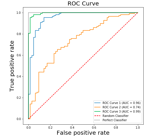
The Receiver Operating Characteristic (ROC) curve is a graph that visualizes this trade-off. It plots the True Positive Rate (y-axis) against the False Positive Rate (x-axis) for every possible classification threshold.

Let's continue with the StatQuest video to see exactly how these points come together to form a curve.

After watching, you should understand these key features of the ROC space:

• The Diagonal Line (y=x): This represents a model with no discriminative power—it's equivalent to random guessing. An ROC curve below this line means the model is performing worse than random.
• The Top-Left Corner (FPR=0, TPR=1): This is the ideal point. It represents a perfect classifier that identifies all positive cases (TPR=1) without making any false positive errors (FPR=0).
• The Curve: A good model's ROC curve will "bow" up towards the top-left corner. The more it bows, the better the model's ability to distinguish between the positive and negative classes.

AUC: Summarizing Performance in a Single Number

Looking at a curve is insightful, but what if we want to compare two different models? It can be hard to tell which curve is "better" just by looking. This is where the Area Under the Curve (AUC) comes in.

The AUC is a single scalar value that measures the entire two-dimensional area underneath the ROC curve.

Here's how to interpret the AUC score:

• AUC = 1.0: Represents a perfect classifier.
• AUC = 0.5: Represents a model with no discriminative ability (equivalent to random guessing).
• AUC > 0.5: The model has some ability to distinguish between classes. A higher AUC generally indicates a better model.
• AUC < 0.5: The model is performing worse than random. This is rare, and often suggests an error in your code or that the model's predictions are inverted.

A useful intuitive interpretation is that the AUC is the probability that the model will rank a randomly chosen positive instance higher than a randomly chosen negative instance.

Plotting ROC and AUC in Python

Now let's put this into practice. scikit-learn provides all the tools we need to easily generate ROC curves and calculate AUC scores for one or more models.

The article below provides a clear, step-by-step guide with code.

Here is a consolidated code example based on the article that you can run. It trains a Logistic Regression and a Random Forest model and plots their ROC curves on the same graph for comparison.

import matplotlib.pyplot as plt
from sklearn.datasets import make_classification
from sklearn.model_selection import train_test_split
from sklearn.linear_model import LogisticRegression
from sklearn.ensemble import RandomForestClassifier
from sklearn.metrics import roc_curve, roc_auc_score

# 1. Generate a binary classification dataset
X, y = make_classification(n_samples=1000, n_features=20, n_classes=2, random_state=42)

# 2. Split into training and testing sets
X_train, X_test, y_train, y_test = train_test_split(X, y, test_size=0.3, random_state=42)

# 3. Define and train the models
models = {
    "Logistic Regression": LogisticRegression(),
    "Random Forest": RandomForestClassifier(random_state=42)
}

# 4. Plot the ROC curves
plt.figure(figsize=(10, 8))

for name, model in models.items():
    # Train the model
    model.fit(X_train, y_train)

    # **Key Step**: Get the probability scores for the positive class
    # The output of predict_proba is [prob_class_0, prob_class_1] for each sample.
    # We need the probabilities for the positive class (class 1).
    y_probs = model.predict_proba(X_test)[:, 1]

    # Calculate the ROC curve and AUC score
    fpr, tpr, thresholds = roc_curve(y_test, y_probs)
    auc_score = roc_auc_score(y_test, y_probs)

    # Plot the curve
    plt.plot(fpr, tpr, lw=2, label=f'{name} (AUC = {auc_score:.2f})')

# 5. Plot the random guessing line and customize the plot
plt.plot([0, 1], [0, 1], color='navy', lw=2, linestyle='--')
plt.xlim([0.0, 1.0])
plt.ylim([0.0, 1.05])
plt.xlabel('False Positive Rate')
plt.ylabel('True Positive Rate')
plt.title('ROC Curve Comparison')
plt.legend(loc="lower right")
plt.grid(True)
plt.show()

This code produces a single plot that lets you visually compare the performance of the two models across all thresholds, with their overall performance neatly summarized by the AUC score in the legend.

Conclusion

Congratulations on completing this lesson and the classification module! You now have a powerful and nuanced way to evaluate and compare your classification models.

Key Takeaways:

• ROC curves visualize the trade-off between the True Positive Rate (TPR) and False Positive Rate (FPR) across all possible classification thresholds.
• A model's performance is better the more its ROC curve "bows" towards the top-left corner (high TPR, low FPR).
• The Area Under the Curve (AUC) provides a single number from 0 to 1 to summarize a model's overall discriminative ability, making it excellent for model comparison. An AUC of 1.0 is perfect, while 0.5 is no better than random guessing.
• In Python, you use model.predict_proba(), roc_curve(), and roc_auc_score() from scikit-learn to get the necessary data for plotting.

Preview of the Next Lesson:

We have now covered the essentials of Supervised Learning for both regression and classification. In the next module, we will venture into a different paradigm of machine learning: Unsupervised Learning. We will start by exploring a fundamental technique for Dimensionality Reduction called Principal Component Analysis (PCA), which helps us simplify and understand complex, high-dimensional datasets.