t-SNE for Dimensionality Reduction

The Core Idea: Preserving Neighborhoods

Imagine you have a complex dataset with many features, like images of handwritten digits. In the original high-dimensional space (e.g., 64 dimensions for an 8x8 image), some digits are "closer" to each other (e.g., a '1' is more similar to a '7' than to an '8').

t-SNE's goal is to arrange all the data points on a 2D plot such that their neighborhood relationships are preserved. Points that were close neighbors in the high-dimensional space should end up as close neighbors on the 2D plot.

To build an intuition for this, let's watch an excellent explanation from StatQuest.

As the video explains, t-SNE models the data as a system of points with forces acting between them.

• Attraction: Similar points (close in high-dimensional space) attract each other.
• Repulsion: Dissimilar points (far apart in high-dimensional space) repel each other.

The algorithm iteratively adjusts the positions of points on the 2D map until it finds a stable configuration where these forces are balanced.

How t-SNE Works: The Mathematical Foundation

Given your background in computer science and math, you'll appreciate understanding the mechanism behind this process. t-SNE operates in three main stages. This next resource provides an excellent, in-depth explanation.

Let's summarize the key ideas from that reading:

1. Measuring Similarities in High-Dimensional Space:

   • t-SNE doesn't use raw distances. Instead, it converts the Euclidean distances between points into conditional probabilities, representing similarities.
   • For each point, it places a Gaussian (normal) distribution around it. The probability of another point being its "neighbor" is proportional to its density under this Gaussian curve.
   • This means nearby points get a high similarity probability, and distant points get a very low one.
   • The perplexity hyperparameter you'll soon encounter is used here; it controls the variance (width) of this Gaussian, effectively defining the size of the local neighborhood for each point.

2. Measuring Similarities in Low-Dimensional Space:

   • The algorithm randomly scatters the points on a 2D map and measures similarities there as well.
   • Crucially, it does not use a Gaussian distribution here. It uses a Student's t-distribution with one degree of freedom. This distribution has "heavier tails" than a normal distribution.
   • Why? This is the key to avoiding the "crowding problem." The heavier tails allow dissimilar points to be placed further apart in the 2D map without incurring a huge penalty, giving the clusters more room to "breathe" and form distinct groups. This is the "t" in t-SNE.

3. Minimizing the Difference:

   • Now we have two sets of probabilities: the target similarities from the high-dimensional space (p_ij) and the current similarities in our 2D map (q_ij).
   • t-SNE uses a cost function called Kullback-Leibler (KL) Divergence to measure the difference between these two distributions.
   • The goal is to adjust the positions of the points in the 2D map to minimize this KL divergence. This is an optimization problem solved using gradient descent, iteratively nudging the points until the low-dimensional similarities (q_ij) faithfully reflect the high-dimensional ones (p_ij).

Implementing t-SNE with Scikit-Learn

Now for the practical part. Scikit-learn's TSNE class makes applying this powerful algorithm straightforward. We will use the load_digits dataset, which contains 64-dimensional data representing 8x8 images of handwritten digits.

The following resource provides a complete, well-commented walkthrough. We will follow its steps and analyze the code.

Let's break down the code and key concepts from the article.

Step 1: Load and Prepare Data

As with PCA, t-SNE is based on distances, so it's sensitive to feature scales. Standardizing the data is a critical first step.

from sklearn.datasets import load_digits
from sklearn.preprocessing import StandardScaler
from sklearn.manifold import TSNE
import matplotlib.pyplot as plt
import numpy as np
import seaborn as sns

# Load the digits dataset
digits = load_digits()
X = digits.data
y = digits.target

print(f"Original data shape: {X.shape}") # (1797 samples, 64 features)

# Standardize the data
scaler = StandardScaler()
X_scaled = scaler.fit_transform(X)

Step 2: Apply t-SNE

We instantiate the TSNE object and then call fit_transform().

# Apply t-SNE
tsne = TSNE(n_components=2, perplexity=30, learning_rate=200, random_state=42)
X_tsne = tsne.fit_transform(X_scaled)

print(f"Embedded data shape: {X_tsne.shape}") # (1797 samples, 2 components)

Key Hyperparameters:

• n_components: The dimension of the embedded space (usually 2 for visualization).
• perplexity: This is the most important parameter. It relates to the number of nearest neighbors that each point considers. Typical values are between 5 and 50. It heavily influences what the final plot looks like.
• learning_rate: The step size for the gradient descent optimizer. Typical values are between 10 and 1000. Scikit-learn's default (200) is often a good starting point.
• random_state: t-SNE has a random initialization step. Setting this ensures your results are reproducible. Always use this!

Step 3: Visualize the Results

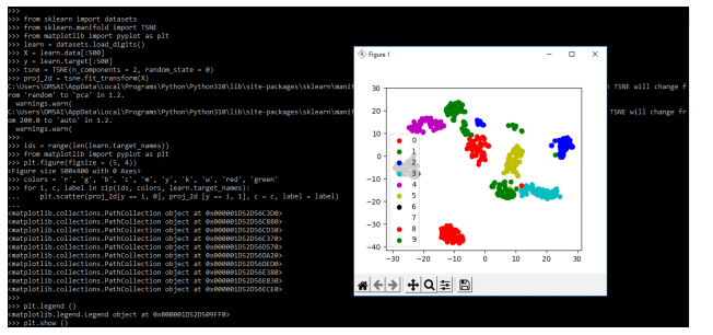
The output X_tsne is a NumPy array with two columns, which we can plot as a scatter plot. We color the points by their true labels (y) to see if t-SNE successfully grouped similar digits.

# Visualize the t-SNE embedding
plt.figure(figsize=(12, 10))
sns.scatterplot(
    x=X_tsne[:, 0], y=X_tsne[:, 1],
    hue=y,
    palette=sns.color_palette("hsv", 10),
    legend="full",
    alpha=0.8
)
plt.title('t-SNE Visualization of Digits Dataset')
plt.xlabel('t-SNE Component 1')
plt.ylabel('t-SNE Component 2')
plt.legend(title='Digit')
plt.show()

When you run this code, you'll see a beautiful plot where the digits are separated into distinct, well-defined clusters. This is a powerful demonstration of t-SNE's ability to find structure in high-dimensional data.

How to Interpret t-SNE Plots: Best Practices and Pitfalls

t-SNE is powerful, but it's also easy to misinterpret. The visualizations can be so compelling that we might read more into them than is actually there.

Please review these essential guidelines to use t-SNE effectively and responsibly.

Here are the most important rules to remember:

• Cluster sizes mean nothing. The area a cluster occupies in a t-SNE plot is not proportional to the size of the cluster in the original data.
• Distances between clusters may not mean anything. Two clusters that are far apart are not necessarily "more different" than two clusters that are closer together. t-SNE preserves local neighborhoods, not global distances.
• t-SNE is for visualization, not analysis. Unlike PCA, the axes of a t-SNE plot do not have a clear interpretation. You cannot use t-SNE to reduce features for a machine learning model, as it doesn't learn a function to transform new data. It's a tool for exploration.
• Run it multiple times. Due to its random initialization, you might get slightly different plots on different runs. It's good practice to run it a few times to ensure the observed clusters are stable and not just an artifact of a lucky initialization.

Conclusion

In this lesson, we've added a powerful non-linear visualization technique to your toolkit. We've seen how t-SNE can take a high-dimensional dataset and produce an intuitive 2D map that reveals the underlying structure.

Key Takeaways:

• t-SNE is a non-linear dimensionality reduction technique primarily used for data visualization.
• It works by preserving local neighborhood structures, ensuring that points close in high-dimensional space remain close in the 2D map.
• It uses probability distributions (Gaussian in high-dim, t-distribution in low-dim) and minimizes the KL divergence between them.
• The perplexity hyperparameter is crucial and should be tuned to find the most meaningful visualization, balancing local and global detail.
• Interpreting t-SNE plots requires care: do not assign meaning to cluster sizes or the distances between clusters.

Preview of the Next Lesson:

Now that we have two powerful tools for exploring and visualizing data (PCA and t-SNE), we are ready to dive deeper into unsupervised learning. In our next lesson, we will learn how to automatically find groups in our data using one of the most famous clustering algorithms: K-Means Clustering. You'll find that t-SNE is an excellent companion to clustering, as it allows you to visualize the clusters your algorithm has found.