Understanding Loss Landscapes in Deep Learning

Introduction

In our recent lessons, we have assembled a powerful toolkit for training deep neural networks, covering optimizers like Adam, regularization via dropout, and stabilization with batch normalization. We've focused on the how of training. Now, we will explore the why by delving into the geometry of the optimization problem itself. This will provide a much deeper, theoretical understanding of the challenges and successes we observe during training.

This lesson introduces the concept of the loss landscape, the high-dimensional surface that our optimization algorithms navigate. We will analyze the critical features of this landscape—local minima and saddle points—and investigate their profound impact on the training process. You will learn why the conventional wisdom about getting stuck in local minima is insufficient for deep learning, and why saddle points represent a more significant challenge. Finally, we will explore the qualitative differences between minima and see how the shape of the landscape is not just a mathematical curiosity, but is deeply connected to a model's ability to generalize to new data.

The Geometry of Optimization: Loss Landscapes

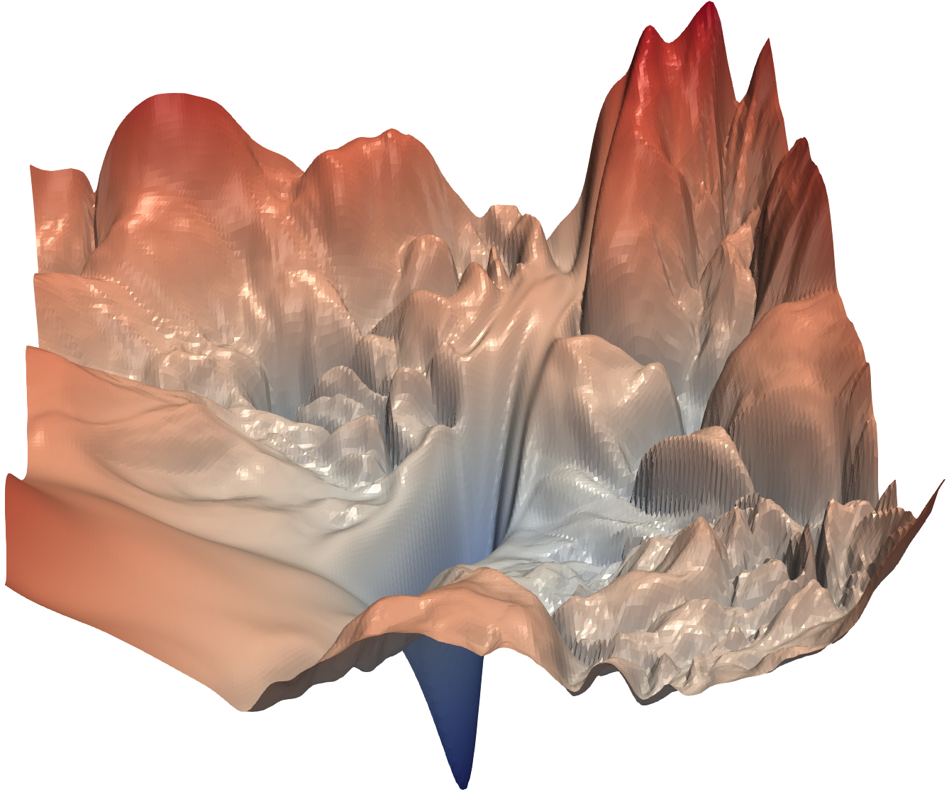
Training a neural network involves finding a set of parameters (weights and biases) $\theta$ that minimizes a loss function $L(\theta )$. We can visualize this process as an optimization algorithm descending a complex surface, where the dimensions are the parameters of the network and the height at any point is the corresponding loss. This surface is the loss landscape.

For a network with millions of parameters, this landscape exists in a million-dimensional space, which is impossible to visualize directly. However, by studying 2D and 3D cross-sections, we can build powerful intuitions about its structure.

To analyze this terrain mathematically, we can use a second-order Taylor expansion to approximate the loss function $L$ around a point $\theta$:

$$L(\theta +\Delta \theta )\approx L(\theta )+\nabla L(\theta {)}^T\Delta \theta +\frac{1}{2}\Delta {\theta }^{T}H\Delta \theta$$

Here, $\nabla L(\theta )$ is the gradient, which we know points in the direction of steepest ascent. The new term, $H$, is the Hessian matrix, which is the matrix of second-order partial derivatives. For a network with $N$ parameters, it is an $N\times N$ matrix:

$$H_{ij}=\frac{{\partial }^{2}L}{\partial {\theta }_i\partial {\theta }_j}$$

The Hessian describes the curvature of the loss landscape. Its eigenvectors point along the principal axes of curvature, and its eigenvalues indicate how steep or flat the landscape is in those directions. A positive eigenvalue corresponds to a direction that curves upwards (like a valley), while a negative eigenvalue corresponds to a direction that curves downwards (like a ridge).

The following video lecture provides a good foundation for understanding how the Hessian characterizes the landscape, using the more intuitive case of multivariate quadratic functions.

The landscapes for simple models like linear or logistic regression are convex: they have a single, bowl-like shape where any local minimum is also the global minimum. Gradient descent is guaranteed to find this minimum. However, the loss landscapes of neural networks are highly non-convex due to the nested non-linear activation functions. This non-convexity is the source of our optimization challenges.

Local Minima vs. Saddle Points: The Real Obstacle

For decades, a primary concern in non-convex optimization was the presence of numerous local minima—points that are optimal within their immediate neighborhood but have a higher loss than the global minimum. The fear was that an optimizer like gradient descent would get trapped in a poor-quality local minimum, leading to a suboptimal model.

However, research in the last decade has revealed a more nuanced picture. In the extremely high-dimensional spaces of deep learning:

1. Most local minima are of surprisingly high quality, with loss values very close to that of the global minimum.
2. The far more prevalent and problematic features are saddle points.

A saddle point is a critical point (where the gradient is zero) that is a minimum along some dimensions (positive Hessian eigenvalues) and a maximum along others (negative Hessian eigenvalues). Imagine the center of a horse's saddle: you can go down towards the stirrups or up towards the front and back.

Why do saddle points dominate in high dimensions? The following paper provides the core theoretical argument, drawing from random matrix theory.

The theoretical insight is that for a point to be a local minimum, the curvature must be positive in all $N$ dimensions. The probability of this happening by chance decreases exponentially with $N$. In contrast, a saddle point only requires a mix of positive and negative curvatures, which becomes overwhelmingly probable as $N$ grows.

Furthermore, these saddle points are often surrounded by extensive, high-error plateaus where the curvature is very low (eigenvalues are close to zero). In these regions, the gradient is tiny, causing first-order methods like standard gradient descent to slow to a crawl, creating the illusion of being stuck in a local minimum. This is often what a "plateau" in your training loss graph signifies.

Fortunately, the optimizers we have studied are well-equipped to handle saddle points:

• Stochastic Gradient Descent (SGD): The noise inherent in using mini-batches provides random perturbations. If the optimizer is on a plateau, this noise can "kick" the parameters into a direction of negative curvature, allowing it to "roll off" the saddle.
• Momentum: By accumulating velocity, momentum-based optimizers can coast through flat plateau regions and escape the saddle, even when the current gradient is very small.

The Quality of Minima: Flatness, Sharpness, and Generalization

While poor local minima may be rare, not all minima are created equal. A key discovery in deep learning is that the geometry of a minimum is strongly correlated with the model's generalization performance. We can categorize minima as:

• Flat Minima: These correspond to wide, open valleys in the loss landscape. They are characterized by small eigenvalues of the Hessian (low curvature).
• Sharp Minima: These are narrow, steep ravines, characterized by large Hessian eigenvalues (high curvature).

The prevailing theory is that flat minima generalize better. The intuition is that the training and test data distributions are slightly different. This difference can be thought of as a small perturbation to the model's parameters $\theta$. If the model is in a flat minimum, a small change in $\theta$ does not lead to a large increase in loss. If it's in a sharp minimum, the same small change can cause a catastrophic spike in loss. Flat minima are therefore more robust.

The type of minimum an optimizer finds is influenced by the training process:

• Large Batch Sizes tend to find sharper minima.
• Small Batch Sizes, with their inherent noise, are better at finding and settling into wider, flatter minima.
• Adaptive optimizers like Adam are sometimes observed to converge to sharper solutions than SGD with momentum.

Most strikingly, architectural choices have a dramatic effect on the overall smoothness of the loss landscape. Networks with skip connections, such as Residual Networks (ResNets), produce vastly smoother landscapes than simple deep networks (like VGG). This is a primary reason why they are so much easier to train.

The following talk by Tom Goldstein provides a compelling visual demonstration of this phenomenon.

This discovery is a powerful example of how theoretical understanding of the optimization geometry can inform practical architecture design. The effectiveness of ResNets isn't just an empirical accident; it is rooted in their ability to fundamentally reshape the problem that our optimizers are trying to solve.

Conclusion

This lesson has taken us on a tour of the geometric world of deep learning optimization. By understanding the topography of the loss landscape, we can better interpret the behavior of our training algorithms.

The key takeaways are:

• Deep learning optimization is the navigation of a high-dimensional, highly non-convex loss landscape. The local curvature of this landscape is described by the Hessian matrix.
• Contrary to earlier intuition, the primary obstacles to optimization in high dimensions are saddle points surrounded by plateaus, not poor-quality local minima.
• Stochasticity (from SGD) and velocity (from momentum) are effective mechanisms for escaping saddle points.
• The geometry of the solution matters: flat minima are more robust to shifts in data distribution and tend to generalize better than sharp minima.
• Architectural innovations, most notably skip connections in ResNets, have a profound impact by making the loss landscape significantly smoother and easier to optimize.

This concludes our module on the principles of training and regularizing deep neural networks. You now have a comprehensive understanding of not just the tools of the trade, but also the theoretical reasons for their effectiveness. In the next module, we will apply these principles as we explore powerful, specialized architectures, beginning with Convolutional Neural Networks for processing spatial data.