Batch Normalization: Theory and Practice

Introduction

Welcome to our next lesson on the essential techniques for training deep neural networks. In our previous session, we examined dropout, a clever regularization method that prevents overfitting by stochastically deactivating neurons during training. Now, we turn our attention from regularization to another fundamental challenge: the stability and speed of the training process itself.

This lesson introduces Batch Normalization (BN), a technique that has become a standard component in most modern deep learning architectures. We will explore its mechanism, the problem it was originally designed to solve—known as internal covariate shift—and the critical differences in its behavior during the training and inference phases. Finally, we will go beyond the original paper's hypothesis to discuss the modern understanding of why Batch Normalization is so effective.

The Problem: Internal Covariate Shift

Training a very deep neural network is notoriously difficult. As training progresses, the weights in each layer are updated. This means that the distribution of the inputs to a subsequent layer is constantly changing. For example, the distribution of activations fed into layer 4 will change every time the weights in layers 1, 2, and 3 are updated.

The original authors of Batch Normalization termed this phenomenon Internal Covariate Shift (ICS). Each layer in the network is essentially trying to learn from a moving target, continuously adapting to a new input distribution from the preceding layer. This instability creates several problems:

• It forces the use of very small learning rates to prevent the training process from becoming unstable or diverging.
• It makes the network highly sensitive to the initial values of the weights.
• It can cause neurons with saturating activation functions (like the sigmoid) to get "stuck" in their saturated regions, where gradients are close to zero, effectively halting learning.

To understand the authors' original motivation, let's turn to the seminal paper that introduced this concept.

The core idea proposed to solve this is deceptively simple: what if we could force the distribution of each layer's inputs to remain more stable throughout training?

The Mechanism of Batch Normalization

Batch Normalization addresses ICS by explicitly normalizing the inputs to a layer. The "batch" in the name refers to the fact that this normalization is performed using the statistics (mean and variance) of the current mini-batch of data.

The process is typically applied to the pre-activations, $z$, which are the linear outputs of a layer before the non-linear activation function is applied. For a mini-batch of $m$ examples, the BN algorithm performs the following steps for each feature (or neuron output) independently:

1. Calculate Mini-Batch Mean: Compute the mean of the activations for the current mini-batch.
   ${\mu }_{\mathcal{B}}=\frac{1}{m}{\sum }_{i=1}^m{z}_i$

2. Calculate Mini-Batch Variance: Compute the variance of the activations for the current mini-batch.
   ${\sigma }_{\mathcal{B}}^2=\frac{1}{m}{\sum }_{i=1}^m(z_i-{\mu }_{\mathcal{B}}{)}^2$

3. Normalize: Normalize each activation using the mini-batch mean and variance. A small constant $ϵ$ is added for numerical stability to avoid division by zero.
   ${\hat{z}}_i=\frac{z_i-{\mu }_{\mathcal{B}}}{\sqrt{{\sigma }_{\mathcal{B}}^2+ϵ}}$
   At this point, the activations ${\hat{z}}_i$ for the mini-batch have a mean of approximately 0 and a variance of 1.

4. Scale and Shift: Simply forcing the activations to a standard normal distribution could limit the network's expressive power. For example, for a sigmoid activation function, this would constrain the inputs to its linear regime. To overcome this, BN introduces two new learnable parameters for each feature: a scale parameter $\gamma$ and a shift parameter $\beta$. The final output of the BN layer is:
   $y_i=\gamma {\hat{z}}_i+\beta$

These parameters $\gamma$ and $\beta$ are learned via backpropagation along with the network's weights. They allow the network to learn the optimal mean and variance for each layer's inputs. In the extreme case, if the network determines that the original activations were best, it can learn to set $\gamma =\sqrt{{\sigma }_{\mathcal{B}}^2+ϵ}$ and $\beta ={\mu }_{\mathcal{B}}$, effectively recovering the identity transformation.

The following video provides a clear walkthrough of this process.

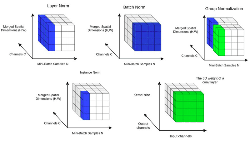
When visualized across a data tensor (N, C, H, W for images), Batch Norm computes its statistics across the batch dimension (N) for each channel (C), as shown below.

The Critical Distinction: Training vs. Inference

The dependency on mini-batch statistics creates a crucial difference between how Batch Normalization operates during training versus during inference (or testing).

During Training: We use the mean and variance of the current mini-batch to perform the normalization, as described above.

During Inference: We often want to make a prediction for a single input example. In this case, a "mini-batch" of size one has a meaningless variance of zero. Furthermore, we need the model's output to be deterministic for a given input; it shouldn't depend on what other inputs are processed alongside it.

The solution is to use an estimate of the entire training set's population statistics. During the training phase, BN layers not only calculate mini-batch statistics but also maintain an exponentially moving average of the mean and variance seen across all mini-batches.

${\mu }_{population}\leftarrow \text{momentum}\times {\mu }_{population}+(1-\text{momentum})\times {\mu }_{\mathcal{B}}$
${\sigma }_{population}^2\leftarrow \text{momentum}\times {\sigma }_{population}^2+(1-\text{momentum})\times {\sigma }_{\mathcal{B}}^2$

At inference time, these fixed, pre-computed population statistics are used in the normalization step instead of mini-batch statistics. The BN layer effectively becomes a simple linear transformation, applying a fixed scale and shift to the activations.

This distinction is fundamental to understanding and correctly implementing BN.

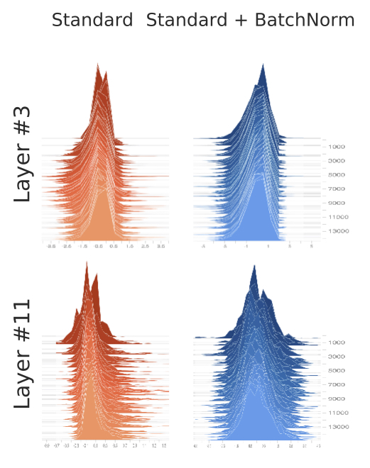
The visual effect of Batch Normalization is striking. The distributions of activations in deeper layers remain much more stable throughout training, preventing the erratic shifts and saturation seen in standard networks.

Why Does Batch Normalization Really Work?

For several years after its publication, the reduction of Internal Covariate Shift was the accepted explanation for BN's success. However, subsequent research has challenged this view. A 2018 paper titled "How Does Batch Normalization Help Optimization?" showed that even in the presence of significant internal covariate shift, BN still improved performance. They also found that BN's impact on the stability of layer input distributions was not as significant as previously believed.

This has led to a new, more widely accepted hypothesis: Batch Normalization works primarily by smoothing the optimization landscape.

What does this mean?

• The loss surface becomes less "jagged" and more predictable. This makes the gradient a more reliable estimate of the direction of steepest descent.
• By making the landscape smoother, BN allows for the use of much higher learning rates, dramatically accelerating convergence. With a jagged landscape, a large learning rate step could easily "overshoot" a minimum and land in a region of high loss, causing instability. On a smoother surface, larger steps are safer.
• It makes the performance of gradient descent less dependent on the initial parameter values.

In addition to this primary effect, BN also provides a mild regularization benefit. The noise introduced by using mini-batch statistics (which are only an estimate of the true population statistics) for normalization at each step prevents the network from relying too heavily on any single training example, similar to the effect of dropout.

This evolution in understanding is a fantastic example of the scientific process within the machine learning field. An initial hypothesis (reducing ICS) explained an observed phenomenon (faster training) and led to a powerful technique, but further investigation revealed a deeper, more fundamental reason for its effectiveness (smoothed optimization landscape).

Conclusion

In this lesson, we have dissected Batch Normalization, a technique that is indispensable for training today's deep neural networks. It not only accelerates training but also makes it more stable and less sensitive to hyperparameter choices.

Here are the key takeaways:

• Mechanism: BN normalizes the pre-activations of a layer using the mean and variance of the current mini-batch, followed by a learnable scale ($\gamma$) and shift ($\beta$) to preserve the network's representational power.
• Original Hypothesis: It was proposed to solve the problem of Internal Covariate Shift, where the changing distributions of layer inputs slow down and destabilize training.
• Training vs. Inference: BN operates differently in these two modes. It uses mini-batch statistics for training and fixed, pre-computed population statistics (via moving averages) for deterministic inference.
• Modern Understanding: The primary benefit of BN is now understood to be its effect on smoothing the loss landscape, which enables the use of higher learning rates and leads to faster, more stable convergence. It also provides a secondary regularization effect.

With your understanding of advanced optimizers, dropout, and now batch normalization, you have a solid grasp of the core toolkit for training deep networks. In our next lesson, we will delve deeper into the geometry of deep learning, analyzing the structure of loss surfaces and the roles of local minima and saddle points in the optimization process.