Momentum Optimization: Speeding Up Convergence

Introduction

In our previous lesson, we established Stochastic Gradient Descent (SGD) as a computationally efficient method for navigating the loss landscape of a neural network. However, we also identified its primary drawback: the noisy, oscillating path it takes towards a minimum, which can slow convergence, particularly in the elongated, high-curvature valleys typical of ill-conditioned problems.

This lesson addresses that inefficiency head-on. We will explore momentum-based optimization, a powerful technique that enhances SGD by incorporating a memory of past updates. The central learning outcome is to explain this method and its physical analogy for accelerating convergence. We will begin with the popular "heavy ball" intuition, formalize the mathematics behind it, and then delve into a more precise physical model—the damped harmonic oscillator. Finally, we'll briefly examine Nesterov Accelerated Gradient (NAG), a popular and effective refinement of the core momentum concept.

The Problem with SGD and the Intuition of Momentum

Recall the "zigzag" path of SGD. When descending a steep, narrow valley in the loss landscape, the gradient points almost perpendicularly across the valley floor. SGD takes a step in this direction, overshoots, and on the next iteration, the gradient points back across the valley. The result is a series of slow, oscillating steps, with only minor progress along the valley's main axis.

Momentum aims to solve this by smoothing out the updates. Instead of relying solely on the current gradient, it accumulates an exponentially decaying moving average of past gradients. This has two effects:

1. Damping Oscillations: In directions where the gradient repeatedly flips sign (like crossing the narrow valley), the averaging process cancels these oscillations out.
2. Accelerating Progress: In directions where the gradient is consistent (like moving down the valley floor), the successive updates build on each other, gathering speed.

The following video provides an excellent visual and intuitive explanation of this process.

The Physical Analogy: A Heavy Ball Rolling Downhill

A powerful and common analogy for momentum is that of a heavy ball rolling down the loss surface.

• Standard GD/SGD: This is like a person walking down the hill, meticulously following the direction of steepest descent at every single point. They change direction instantly but may make slow progress in winding valleys.
• Momentum: This is like a heavy ball. Its inertia (momentum) prevents it from making sharp turns. It smooths out its path, resists the urge to zigzag across a ravine, and builds up speed as it barrels down a consistent slope.

In this analogy:

• The gradient ($\nabla J$) acts as a force, providing acceleration.
• The velocity ($v$) is accumulated over time.
• A friction term (the momentum coefficient) prevents the ball from accelerating indefinitely.

Let's watch a brief segment that formalizes this analogy.

Mathematical Formulation and Theoretical Analysis

The most common implementation of what is now called "Classical Momentum" (CM) uses a velocity vector, $v$, which is an exponentially weighted moving average of the gradients. The update rules at step $t$ are:

1. Update velocity: $$v_t=\beta v_{t-1}+(1-\beta ){\nabla }_{\theta }J({\theta }_{t-1})$$
2. Update parameters: $${\theta }_t={\theta }_{t-1}-\alpha v_t$$

Here:

• $\theta$ are the model parameters.
• $\alpha$ is the learning rate.
• $\beta$ is the momentum coefficient (a common value is 0.9). It controls the decay rate of past gradients' influence. A higher $\beta$ means past gradients are "remembered" for longer.
• $v_t$ is the velocity vector at time $t$.

(Note: An alternative but equivalent formulation, which you will see in some literature, combines the learning rate into the velocity update: $v_t=\beta v_{t-1}+\alpha {\nabla }_{\theta }J({\theta }_{t-1})$. The version above is often preferred as it decouples the momentum and learning rate hyperparameters.)

To truly understand why this works, we must go beyond the analogy and analyze its dynamics mathematically. A standard approach, which leverages your background in linear algebra, is to study the algorithm's behavior on a quadratic objective function, $f(x)=\frac{1}{2}{x}^{T}Sx$, where $S$ is a positive definite symmetric matrix (the Hessian). Since any general smooth loss function is locally quadratic near a minimum, this analysis provides powerful insights.

The following lecture performs this analysis brilliantly. It shows that by introducing momentum, we turn a first-order iterative system into a second-order one. This can be analyzed by converting it into a 2x2 system of first-order equations and studying the eigenvalues of the corresponding iteration matrix.

A Refined Analogy: The Damped Harmonic Oscillator

The mathematical analysis reveals an even more precise physical model than the rolling ball: a damped harmonic oscillator. This is the classic physics problem of a mass attached to a spring, with friction.

The Distill article "Why Momentum Really Works" provides an elegant explanation of this connection.

Nesterov Accelerated Gradient (NAG)

A popular and often superior variant of momentum is Nesterov Accelerated Gradient (NAG), introduced by Yurii Nesterov in 1983. It introduces a subtle but impactful change.

• Classical Momentum (CM): First, it computes the gradient at the current position (${\theta }_t$). Then, it takes a large "momentum step" in the direction of the accumulated velocity $v_t$.
• Nesterov Momentum (NAG): First, it takes the momentum step to a temporary, "look-ahead" position (${\theta }_t-\alpha \beta v_{t-1}$). Then, it computes the gradient at that future position to make a correction.

This "look-ahead" feature acts as a smarter correction mechanism. If the momentum step is about to overshoot, the gradient at the look-ahead point will be stronger in the opposite direction, providing a more responsive brake and leading to more stable convergence.

The update rules for NAG can be written as:

1. Update velocity: $$v_t=\beta v_{t-1}+(1-\beta ){\nabla }_{\theta }J({\theta }_t-\alpha \beta v_{t-1})$$
2. Update parameters: $${\theta }_t={\theta }_{t-1}-\alpha v_t$$

The following image provides a clear vector diagram illustrating the difference.

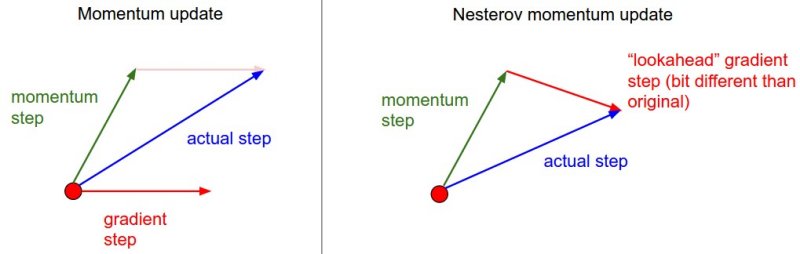
For a formal discussion of this difference, the paper that helped popularize momentum in deep learning provides a concise explanation.

Conclusion

In this lesson, we have moved beyond simple SGD to a more sophisticated optimization technique. We have seen how momentum accelerates learning by intelligently navigating the loss landscape.

Your key takeaways are:

• Momentum addresses SGD's slow, oscillatory convergence by accumulating an exponentially weighted moving average of past gradients.
• The physical analogy is a heavy ball rolling downhill, where inertia helps smooth the path and build speed. A more precise model is that of a damped harmonic oscillator, where the momentum hyperparameter acts as a damping coefficient.
• The theoretical analysis on quadratic functions reveals that momentum improves the convergence rate dependency on the problem's condition number $\kappa$ to $\sqrt{\kappa }$, a significant acceleration.
• Nesterov Accelerated Gradient (NAG) is an important variant that uses a "look-ahead" gradient calculation to provide better stability and often faster convergence.

So far, we have improved the direction of our gradient steps. However, we have still been using a single, fixed learning rate $\alpha$ for all parameters. What if some parameters need to take large steps while others need to be fine-tuned with small steps? Our next lesson will introduce adaptive learning rate methods, such as RMSProp and Adam, which address exactly this question.