Adaptive Learning Rates: RMSProp vs. Adam

Introduction

In our last lesson, we explored how momentum-based methods improve upon Stochastic Gradient Descent (SGD) by smoothing out the optimization path and accelerating convergence. We saw that by incorporating a "velocity" term—an exponentially weighted moving average of past gradients—we could navigate the narrow, high-curvature valleys of the loss landscape more effectively. However, both SGD and its momentum-based variants still rely on a single, global learning rate $\alpha$ applied uniformly to all model parameters.

This lesson tackles that limitation. We will investigate adaptive learning rate methods, a class of optimizers that compute an individual, per-parameter learning rate. The learning objective is to describe how RMSProp and Adam function as these adaptive methods and to compare their tradeoffs. We will see how they elegantly solve problems that a single learning rate cannot, and why Adam, in particular, has become the de facto standard optimizer for a vast range of deep learning applications.

The Problem: A Single Learning Rate for All

In complex neural networks, not all parameters are created equal. Some parameters may be associated with very frequent features in the data, receiving strong, consistent gradient updates. Others might correspond to rare, sparse features, for which gradients are infrequent and potentially noisy.

Consider a natural language processing model learning word embeddings. The parameter updates for a common word like "the" will be frequent and large, while updates for a rare word like "sesquipedalian" will be few and far between.

• If we set a high global learning rate, we risk the updates for "the" becoming too large, causing oscillations and instability.
• If we set a low global learning rate, the parameters for "the" might converge nicely, but the parameters for "sesquipedalian" will barely update, and the model will fail to learn its meaning.

This motivates the core idea of adaptive methods: what if we could automatically adjust the learning rate for each parameter, slowing it down for parameters with consistently large gradients and speeding it up for those with small or infrequent gradients?

RMSProp: Fixing a Fatal Flaw

The first widely-used adaptive method was AdaGrad (Adaptive Gradient). Its strategy is to scale each parameter's update inversely proportional to the square root of the sum of all its past squared gradients. This means parameters with a history of large gradients get a smaller effective learning rate. While brilliant for sparse data, AdaGrad has a critical issue for deep learning: the sum of squared gradients in the denominator only ever increases. Over time, this causes the learning rate to shrink towards zero, prematurely halting the training process.

RMSProp (Root Mean Square Propagation), proposed by Geoffrey Hinton, provides an elegant fix. Instead of accumulating a sum of all past squared gradients, RMSProp maintains an exponentially weighted moving average (EWMA) of them. This "leaky" accumulator adapts to the most recent gradient information, preventing the learning rate from monotonically decaying to zero.

The algorithm at step $t$ for a single parameter $w$ is:

1. Compute the gradient: $g_t={\nabla }_{w}J(w_t)$
2. Update the moving average of squared gradients, $v_t$: $$v_t=\beta v_{t-1}+(1-\beta )g_t^2$$
3. Update the parameter $w$: $$w_{t+1}=w_t-\frac{\eta }{\sqrt{v_t}+ϵ}{g}_t$$

Here:

• $\eta$ is the master learning rate.
• $\beta$ is the decay rate for the moving average (e.g., 0.9).
• $ϵ$ is a small constant (e.g., $10^{-8}$) to prevent division by zero.

The term $\sqrt{v_t}$ is the "Root Mean Square" of recent gradients that gives the algorithm its name. This term normalizes the gradient: if recent gradients have been large, the denominator is large and the effective step size is small. If recent gradients have been small, the denominator is small and the effective step size is large.

The following video lecture explains this mechanism in detail.

This adaptive behavior is visualized in the image below. In a loss landscape with a narrow valley (steep in the b direction, flat in the w direction), RMSProp dampens the oscillations along the steep b axis and accelerates progress along the flatter w axis, finding a much more direct path to the minimum than standard gradient descent.

Adam: Adaptive Moment Estimation

So far, we've seen two major improvements to SGD:

1. Momentum: Accumulates a moving average of past gradients to accelerate in consistent directions. This is an estimate of the first moment (the mean) of the gradients.
2. RMSProp: Accumulates a moving average of past squared gradients to adapt the per-parameter learning rate. This is an estimate of the second moment (the uncentered variance).

Adam (Adaptive Moment Estimation), proposed by Kingma and Ba, brilliantly combines these two ideas into a single, powerful optimizer. It maintains two separate moving averages: one for the gradients themselves (like momentum) and another for the squared gradients (like RMSProp).

The algorithm proceeds as follows:

1. Compute gradient: $g_t={\nabla }_{w}J(w_t)$
2. Update first moment estimate (momentum): $$m_t={\beta }_1{m}_{t-1}+(1-{\beta }_1)g_t$$
3. Update second moment estimate (RMSProp): $$v_t={\beta }_2{v}_{t-1}+(1-{\beta }_2)g_t^2$$

However, there's a problem. Since $m_0$ and $v_0$ are initialized to zero, in the early steps of training, $m_t$ and $v_t$ are biased towards zero. Adam introduces a crucial bias correction step to counteract this.

4. Compute bias-corrected moment estimates: $${\hat{m}}_t=\frac{m_t}{1-{\beta }_1^t}$$ $${\hat{v}}_t=\frac{v_t}{1-{\beta }_2^t}$$
5. Update parameter: $$w_{t+1}=w_t-\frac{\eta }{\sqrt{{\hat{v}}_t}+ϵ}{\hat{m}}_t$$

The default hyperparameters are typically ${\beta }_1=0.9$, ${\beta }_2=0.999$, and $\eta =0.001$.

The following reading provides a detailed walkthrough of the Adam algorithm and the rationale for its design.

Tradeoffs and Practical Considerations

Adam's combination of momentum and adaptive learning rates makes it incredibly effective and robust across a wide range of problems. It is often the default choice for training deep neural networks.

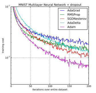
Despite its strengths, Adam is not a silver bullet, and understanding its tradeoffs is crucial for advanced practice.

Generalization vs. Convergence Speed

While Adam converges very quickly, some research has shown that for certain tasks, particularly in computer vision, models trained with SGD+Momentum can achieve slightly better generalization performance on the test set. The theory is that the "noisier" path of SGD helps it settle into "flatter" minima, which are thought to generalize better than the "sharper" minima that Adam might find.

Adam and Regularization: The Rise of AdamW

A critical discovery was that the standard implementation of L2 regularization interacts poorly with adaptive optimizers like Adam. In SGD, adding an L2 penalty to the loss is equivalent to applying weight decay directly to the weights. In Adam, this equivalence breaks. The regularization term in the gradient also gets scaled by the adaptive denominator $1/\sqrt{{\hat{v}}_t}$, meaning parameters with large historical gradients receive less effective regularization.

AdamW (Adam with Decoupled Weight Decay) fixes this. It "decouples" the weight decay from the gradient update. The optimization step is performed using only the gradients from the loss function, and then a separate weight decay step is applied.

• Adam with L2: $w_{t+1}=w_t-\text{AdamUpdate}(\nabla J(w_t)+\lambda w_t)$
• AdamW: $w_{t+1}=w_t-\text{AdamUpdate}(\nabla J(w_t))-\eta \lambda w_t$

This seemingly small change has a significant impact, often leading to better model performance and making AdamW the standard for training state-of-the-art models, especially Transformers.

Conclusion

In this lesson, we have moved from a single, global learning rate to sophisticated, per-parameter adaptive methods. We've traced the evolution of these ideas from the flawed AdaGrad to the robust and powerful Adam optimizer.

Your key takeaways are:

• Adaptive learning rates adjust the step size for each parameter individually, which is crucial for training on data with sparse features and for navigating complex, ill-conditioned loss landscapes.
• RMSProp improves upon AdaGrad by using an exponentially weighted moving average of squared gradients, preventing the learning rate from decaying to zero. It scales updates inversely to the root-mean-square of recent gradients.
• Adam combines the adaptive learning rate mechanism of RMSProp (the second moment) with the velocity of momentum (the first moment). It also introduces a critical bias-correction step to account for the zero-initialization of the moment estimates.
• Tradeoffs: While Adam is a powerful and robust default, it's important to be aware of its potential generalization tradeoffs compared to SGD+Momentum and the critical distinction between L2 regularization and decoupled weight decay, which is correctly handled by AdamW.

We now have a solid understanding of the most important optimization algorithms used in modern deep learning. In our next lesson, we will shift our focus to other essential techniques for successfully training deep networks, starting with dropout, a powerful regularization method, and batch normalization, which helps stabilize the training process.