Training GRUs on Long Streams with Truncated BPTT and Gradient Clipping

Hello! Last lesson gave you a GRU that produces two predictions at every step and carries hidden state across contiguous chunks of one sequence. It deliberately stopped at the forward pass. During training, carrying that state with its entire computation history attached would eventually make a long stream expensive to backpropagate through.

This lesson turns that forward path into a training loop. In about 40–45 minutes, you will learn where to cut the gradient graph without resetting the GRU’s memory, how to apply gradient clipping before an optimizer update, and how to keep unscored steps in the stream.

Keep the state, cut the gradient history

When a GRU processes a chunk, its final hidden state depends on the inputs and parameters used throughout that chunk. If you pass that state directly into the next chunk during training, autograd can trace the next loss back through both chunks. Repeating this across a long sequence defeats the purpose of chunking: earlier activations remain needed for backward computation.

The distinction is subtle but central: the next chunk needs the numerical value of the previous hidden state, not an indefinitely growing path through which to differentiate it. Truncated backpropagation through time, or TBPTT, preserves that value while treating it as a fixed starting state for the next chunk.

Watch how the lecturer separates state handoff from gradient handoff:

For a window of length $K$, losses inside that window can send gradients through its recurrent computations, including contributions to the shared GRU parameters. At the boundary, detaching the outgoing state prevents a later window’s loss from sending gradients into the earlier window. Detaching does not set the state to zero. Information from a distant prefix can still affect later predictions through the state’s value; what is truncated is the later loss’s credit assignment to computations before the boundary.

Dive into Deep Learning gives the mathematical interpretation: truncation drops the older terms from a gradient that would otherwise reach progressively farther into the past.

TBPTT is therefore an approximation, not a way of obtaining the full-sequence gradient using less memory. A longer window permits more distant credit assignment but costs more activation memory and backward time. A shorter window is cheaper but can make dependencies that require long-range parameter updates harder to learn.

Translate the boundary into PyTorch

The PyTorch language-model example demonstrates the two mechanical ingredients: slice a stream along its time dimension and call detach() on the hidden state between slices. Its target is the next token, whereas our targets are two values aligned to specified prediction steps, so we will borrow the mechanics rather than its target construction.

Our previous model accepts state=None for a new independent sequence and returns a state for the next contiguous chunk. Training adds one operation at each chunk boundary:

if state is not None:
    state = state.detach()

predictions, state = model(x_chunk, state)

For a one-layer GRU, state is a tensor shaped $(1,1,H)$ when training one sequence at a time. Do not detach predictions before computing the current chunk’s loss: that would remove the gradient you need. Do not replace state with None at a chunk boundary: that would erase history the next chunk needs.

The lifetime rules are:

• Within one chunk: retain the graph until its loss has been backpropagated.
• At the next chunk boundary: carry the state value, detached from the preceding graph.
• At a true independent-sequence boundary: set state = None.

An unscored or warm-up step still belongs in its chunk’s input. The GRU processes it because it can affect later hidden states, even when its prediction contributes nothing to the loss.

Train on aligned, masked chunks

The validation metric established earlier is a global weighted Pearson score. It is not a sum of independent chunk scores, so computing a separate Pearson correlation for every short chunk is a poor default training objective; a chunk may even have too few eligible targets for a meaningful correlation. We will use masked, weighted mean squared error as a practical training surrogate, then continue to select and assess models with the real chronological validation metric.

For eligible step-and-channel entries $A$, predictions ${\hat{y}}_{t,c}$, targets $y_{t,c}$, and nonnegative weights $w_{t,c}$, the chunk loss is

A step can have one eligible channel and one ineligible channel. The mask therefore has shape $(T,2)$, like the predictions. A chunk with no positive-weight eligible entries still advances hidden state, but supplies no optimizer update.

The following loop uses the TwoOutputGRU from last lesson. It assumes sequence_loader yields one independent, already preprocessed sequence at a time as (x_seq, y_seq, mask_seq, weight_seq), with shapes $(T,F)$, $(T,2)$, $(T,2)$, and $(T,2)$. Inputs and labels are floating-point tensors; masks are Boolean. Eligible weights must be finite and nonnegative, and targets with positive eligible weight must be finite. Ineligible target entries may contain missing values.

import torch


def masked_weighted_mse(pred, target, mask, weight):
    # All tensors have shape (chunk_time, 2).
    # Check the input preconditions when constructing the sequence loader:
    # eligible weights are finite and nonnegative;
    # targets with positive eligible weight are finite.
    active = mask & (weight > 0)

    safe_weight = torch.where(
        active, weight, torch.zeros_like(weight)
    )
    denominator = safe_weight.sum()
    if denominator.item() == 0:
        return None

    # Replace ineligible targets before subtraction: they may be NaN.
    safe_target = torch.where(
        active, target, torch.zeros_like(target)
    )
    return ((pred - safe_target).square() * safe_weight).sum() / denominator


def train_epoch(model, optimizer, sequence_loader, device,
                chunk_len=128, max_norm=1.0):
    model.train()

    for x_seq, y_seq, mask_seq, weight_seq in sequence_loader:
        # This loader item is one independent sequence, not an
        # arbitrary slice that continues a preceding loader item.
        state = None
        sequence_length = x_seq.shape[0]

        for start in range(0, sequence_length, chunk_len):
            stop = min(start + chunk_len, sequence_length)

            x = x_seq[start:stop].unsqueeze(0).to(device)  # (1, K, F)
            y = y_seq[start:stop].to(device)               # (K, 2)
            mask = mask_seq[start:stop].to(device)         # (K, 2)
            weight = weight_seq[start:stop].to(device)     # (K, 2)

            if state is not None:
                state = state.detach()

            optimizer.zero_grad(set_to_none=True)
            pred, state = model(x, state)                   # (1, K, 2)
            loss = masked_weighted_mse(pred[0], y, mask, weight)

            if loss is None:
                # The inputs still updated state. The next iteration
                # will detach it, but there is no update for this chunk.
                continue

            loss.backward()
            pre_clip_norm = torch.nn.utils.clip_grad_norm_(
                model.parameters(),
                max_norm=max_norm,
                error_if_nonfinite=True,
            )
            optimizer.step()

            # Optionally log loss and pre_clip_norm (before clipping).

For example, after moving your model to device, an initial setup could be:

optimizer = torch.optim.AdamW(model.parameters(), lr=1e-3)
train_epoch(model, optimizer, sequence_loader, device,
            chunk_len=128, max_norm=1.0)

These values are starting points, not competition-tuned settings. Adjust the window length to available memory and observed validation behavior. Each optimizer update changes the parameters before the next chunk is processed; together with truncation, this means the loop is not equivalent to one full-sequence forward and backward pass.

Keep the data contract visible while adapting the code. A sequence-sized Parquet row group can supply one loader item without loading the whole dataset into memory, but its rows must remain chronological and its targets and masks must stay aligned. If a loader item is merely the continuation of the same true sequence, resetting at that item would be wrong; the loader must communicate that boundary explicitly. Conversely, adjacent independent sequences must never share state.

Clip the update, not the hidden state

Even within a bounded window, recurrent gradients can occasionally become large. Global-norm clipping limits the magnitude of the parameter-gradient vector immediately after loss.backward() and before optimizer.step(). If all parameter gradients concatenated into a vector $g$ have norm above a threshold $C$, norm clipping approximately applies

Small gradients are left alone; large gradients are scaled together, preserving their relative direction. This differs from capping every gradient element independently. clip_grad_norm_ performs global-norm clipping across the parameters passed to it and returns the pre-clipping norm, which makes pre_clip_norm useful for diagnostics.

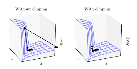
The order in the loop matters. Clipping before backward() has no current gradients to limit, while clipping after optimizer.step() is too late for that update. error_if_nonfinite=True also makes a nonfinite gradient norm fail visibly rather than allowing a suspect update to proceed.

TBPTT and clipping solve different problems. Truncation bounds how far a loss’s gradient graph reaches back and limits activation memory. Clipping limits the size of a computed parameter update. Clipping does not recover gradients that vanish across time, repair nonfinite inputs, or make an overly high learning rate harmless.

As an implementation check, inspect a few training batches for finite losses and log both the loss and the returned pre-clipping norm. If clipping triggers constantly, investigate feature and target scales, loss weighting, and learning rate rather than assuming a lower threshold alone will fix training. Keep these training diagnostics distinct from the masked global validation score.

Takeaways

To train a GRU on a long stream, divide each independent sequence into chronological windows, backpropagate each window’s eligible loss, and detach—not reset—the state passed to the next window. Reset only at a real sequence boundary. Unscored inputs still update state; masks and weights determine which of the two output channels train the model. Clip parameter gradients between backward() and the optimizer step, and evaluate with the actual chronological weighted-Pearson procedure rather than treating the chunk loss as the final metric.

Next, you will compare training and validation behavior across time periods and instruments to diagnose whether this trained sequence model has learned a useful pattern or merely fitted its training streams.