Stateful GRU with Hidden-State Reset and Dual-Step Predictions

Hello! Last lesson established a validation path that keeps sequences intact, resets state at independent boundaries, and scores only eligible predictions. Now we need a model whose outputs can follow that path.

In about 40–45 minutes, you will build a one-layer PyTorch GRU that carries hidden state through a sequence, resets it before a new sequence, and produces two continuous predictions at every step. The scoring mask will decide which of those predictions are required for evaluation; it will not decide whether the GRU processes a step.

What the GRU carries forward

A vanilla RNN compresses its history into a hidden state. A GRU does the same, but uses gates to control how much of that state to retain and how much to revise. Read the gate equations and their interpretation before looking at the implementation.

Using the reading’s convention, the reset gate $r_t$ controls how strongly the previous hidden state participates in forming a candidate state. The update gate $z_t$ then mixes that candidate with the old state:

Here, $\odot$ means elementwise multiplication. When an entry of $z_t$ is near one, that entry largely preserves the old state; when it is near zero, it largely adopts the candidate. Unlike a manual instruction to “remember the last 100 steps,” these are learned, feature-dependent decisions made at each step.

The diagram below is useful for tracing the two routes into the new state. Watch its update-gate convention: it draws the gate value on the candidate route and its complement on the old-state route. The equation above calls the old-state gate value $z_t$. They describe the same mixture if the diagram’s gate is called $1-z_t$; do not combine the two conventions without checking which route a symbol controls. The drawing also omits learned weight operations, so it is a conceptual schematic rather than a literal implementation of nn.GRU.

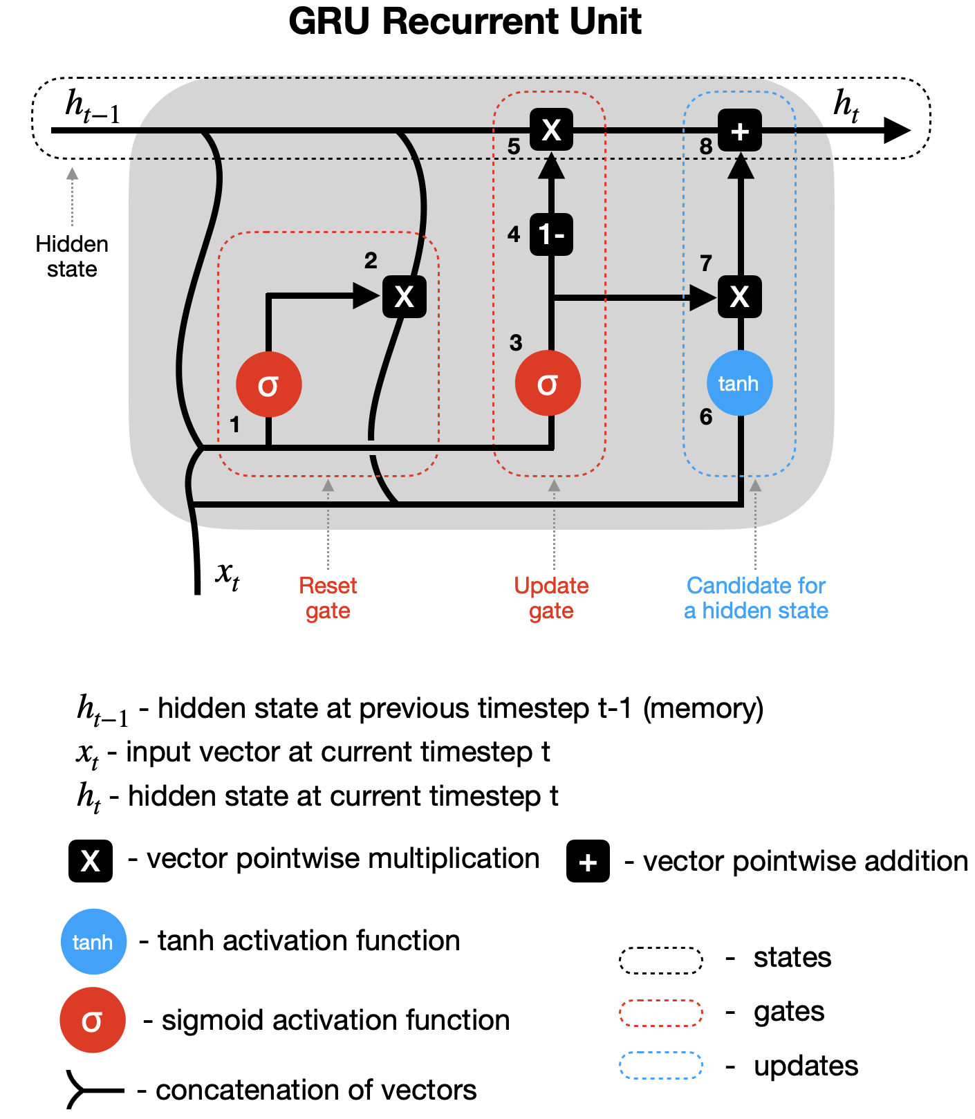
For our task, the consequential fact is the interface: given current features and a previous hidden state, the GRU returns a new hidden state. Its gates learn the recurrence; your code must still manage when a state is carried and when it is reset.

Define the state and output contract

Let a sequence contain $T$ ordered feature vectors, each with $F$ features. We will use batch_first=True, so PyTorch receives an input shaped $(B,T,F)$, where $B$ is the number of independent sequences in a batch. For one GRU layer with hidden width $H$:

• the GRU’s outputs at all steps have shape $(B,T,H)$;
• its final hidden state has shape $(1,B,H)$;
• a linear head applied to all GRU outputs produces $(B,T,2)$.

This differs from sequence classification, where one might keep only the final step. The short video segment below illustrates the PyTorch shape contract and then makes exactly that final-step choice. Watch it as a contrast: we must not discard the earlier steps.

We will call the model stateful because its caller passes the returned state into the next call. We will not hide mutable state inside the nn.Module. An explicit state argument makes resets visible, lets a whole sequence and its smaller chunks use the same model, and avoids accidentally carrying history from one independent sequence into another.

import torch
from torch import nn


class TwoOutputGRU(nn.Module):
    def __init__(self, feature_dim: int, hidden_dim: int):
        super().__init__()
        self.gru = nn.GRU(
            input_size=feature_dim,
            hidden_size=hidden_dim,
            num_layers=1,
            batch_first=True,
        )
        self.head = nn.Linear(hidden_dim, 2)

    def forward(self, x: torch.Tensor, state=None):
        # x: (batch, time, features)
        # state: None, or (1, batch, hidden_dim)
        states_at_steps, next_state = self.gru(x, state)
        predictions = self.head(states_at_steps)
        # predictions: (batch, time, 2)
        return predictions, next_state

There is no softmax: the two outputs are continuous predictions, not probabilities that must sum to one. state=None tells PyTorch to start with a zero hidden state. Passing a previously returned next_state continues from that history. Applying head to the full tensor, rather than to states_at_steps[:, -1, :], is what produces two values at each step.

A sequence-sized row group from the earlier data pipeline can arrive as x_seq with shape $(T,F)$. Add a batch dimension without mixing it with another sequence:

model = TwoOutputGRU(feature_dim=x_seq.shape[1], hidden_dim=64)

predictions, final_state = model(x_seq.unsqueeze(0), state=None)
predictions = predictions[0]  # (T, 2)

The example assumes x_seq is already a suitably preprocessed, floating-point feature tensor. Use training-fitted preprocessing at validation time, as established last lesson. Nothing in the model should infer features from validation targets.

Carry within a sequence; reset between sequences

The distinction between chunks and sequences is an interface invariant. Two consecutive chunks from the same sequence share state. Two independent sequences do not, even if the loader returns them consecutively or they concern the same instrument.

# One independent sequence, divided only to illustrate state handoff.
x = x_seq.unsqueeze(0)       # (1, T, F)
cut = len(x_seq) // 2

first_predictions, state = model(x[:, :cut, :], state=None)
second_predictions, state = model(x[:, cut:, :], state=state)

all_predictions = torch.cat(
    [first_predictions, second_predictions], dim=1
)  # (1, T, 2)

The second call starts where the first left off. If state=None were used for both chunks, the second half would lose its prefix history. Conversely, using that final state for an unrelated sequence would introduce information from the wrong sequence.

A straightforward sequence loop makes the reset explicit:

for x_seq in sequence_loader:  # each item is one independent (T, F) sequence
    state = None               # reset at this true sequence boundary

    x = x_seq.unsqueeze(0)
    predictions, state = model(x, state)

    # Consume predictions[0], shaped (T, 2), alongside this
    # sequence's aligned targets, mask, and weights.

For now, this shows the forward-pass contract, not a training loop. In particular, do not carry a training computation graph indefinitely merely because the forward call accepts state. The next lesson will address long-stream training.

What if the evaluation interface delivers one time step at a time? The same model works with a time dimension of one:

def predict_sequence_online(model, x_seq, required_steps):
    """Yield (step_index, two_predictions) at requested steps.

    x_seq: (T, F), ordered within one independent sequence.
    required_steps: (T,) booleans supplied by the evaluation contract.
    """
    state = None  # a new call represents a new independent sequence

    with torch.no_grad():
        for t in range(len(x_seq)):
            x_step = x_seq[t:t + 1].unsqueeze(0)  # (1, 1, F)
            output, state = model(x_step, state)

            if bool(required_steps[t]):
                yield t, output[0, 0]             # (2,)

Process even an unrequested step. If it is part of the permitted input stream, its features may update the hidden state needed later. required_steps controls which predictions are emitted, not which inputs the GRU sees. If the actual scoring mask is shaped $(T,2)$, its two entries still govern eligibility separately: a step requiring either channel can receive a two-value output, while the scorer excludes any ineligible channel. Do not derive a request flag from unavailable targets, and follow the competition’s actual inference contract if it specifies a different request mechanism.

The timing of features matters as much as the state boundary. A prediction emitted after processing $x_t$ can depend on permitted features through step $t$, not on features from later steps. If the target represents a future horizon, align its label and scoring mask with the step at which the prediction must be made; never shift future feature rows into that input to make tensor shapes line up.

Check the invariants before training

Shape checks catch wiring errors. Equivalence checks catch state errors. In evaluation mode, processing one sequence in a single call, in consecutive chunks, or step by step should give approximately the same predictions when each route starts from the same reset state.

torch.manual_seed(7)

model = TwoOutputGRU(feature_dim=5, hidden_dim=16)
model.eval()
a = torch.randn(9, 5)
b = torch.randn(6, 5)

with torch.no_grad():
    # Reference: one complete independent sequence.
    full, full_state = model(a.unsqueeze(0), state=None)
    assert full.shape == (1, 9, 2)
    assert full_state.shape == (1, 1, 16)

    # Same sequence, split into two consecutive chunks.
    left, state = model(a[:4].unsqueeze(0), state=None)
    right, state = model(a[4:].unsqueeze(0), state=state)
    torch.testing.assert_close(torch.cat([left, right], dim=1), full)
    torch.testing.assert_close(state, full_state)

    # New independent sequence: explicitly reset, despite having full_state.
    b_fresh, _ = model(b.unsqueeze(0), state=None)

required = torch.tensor(
    [False, True, False, True, True, False, False, True, False]
)
selected = list(predict_sequence_online(model, a, required))
assert [t for t, _ in selected] == [1, 3, 4, 7]
for t, pair in selected:
    assert pair.shape == (2,)
    torch.testing.assert_close(pair, full[0, t], atol=1e-6, rtol=1e-5)

# Running a first sequence must not change a freshly reset second sequence.
list(predict_sequence_online(model, a, torch.ones(9, dtype=torch.bool)))
with torch.no_grad():
    b_after_a, _ = model(b.unsqueeze(0), state=None)
torch.testing.assert_close(b_after_a, b_fresh)

The first comparison detects a lost state at a chunk boundary. The stepwise comparison detects incorrect time or output indexing, including the mistake of running only requested steps. The last comparison documents the intended reset boundary. Numerical results can differ slightly across execution paths or devices, so approximate rather than exact equality is appropriate.

During validation, keep the previous lesson’s responsibilities separate. The model returns $(T,2)$ predictions for a sequence; the scorer receives those predictions along with the real aligned targets, channel-level mask, and weights. A masked-out prediction may still have been computed and may still have depended on earlier features. It simply makes no contribution to the score.

Takeaways

A GRU’s hidden state summarizes processed history, while its gates learn how that summary changes. For this task, the implementation contract is more important than hand-coding the gates: apply a two-output head to every GRU step, pass state across contiguous parts of one sequence, and reset it at each independent sequence boundary. Process permitted warm-up or unscored steps so later state is correct; let the scoring mask determine eligibility rather than interrupting the recurrence.

You now have a forward path that can feed the chronological validation pipeline. Next, you will train on long streams without retaining an unbounded computation graph, using truncated backpropagation through time and gradient clipping.