Fermi's Golden Rule and Direct Bandgap Absorption

Hello! Welcome back to our module on the optical properties of solids.

In our last lesson, we explored the Drude model, a classical picture that successfully explains the optical response of free carriers—the so-called intraband response. We saw how it accounts for the high reflectivity of metals and doped semiconductors below their plasma frequency. However, we also noted its limitations: it cannot explain the fundamental absorption edge that defines a semiconductor's transparency window or the characteristic colors of metals like gold and copper.

These phenomena arise from a purely quantum mechanical process: the transition of an electron from an occupied state in one band to an empty state in another. This is called an interband transition. Today, we will develop the theoretical framework to describe this process. Your experience with photoluminescence spectroscopy is highly relevant here, as PL is a direct consequence of the reverse process—an electron falling back across the bandgap and emitting a photon.

Our learning outcome for this lesson is to calculate the optical absorption coefficient for a semiconductor with a direct bandgap using Fermi's golden rule. This will provide us with a quantitative understanding of how and why semiconductors absorb light above a certain energy threshold.

1. The Quantum Mechanical Framework for Absorption

At its heart, optical absorption in a semiconductor is a photon-assisted transition. A photon with energy $\hslash \omega$ is annihilated, and its energy and momentum are transferred to an electron in the valence band, promoting it to an available state in the conduction band. This can only happen if the photon's energy is at least as large as the bandgap, $\hslash \omega \ge E_g$.

To calculate the rate of these transitions, we turn to time-dependent perturbation theory. The central result we need is Fermi's Golden Rule, which gives the transition rate from an initial state $|{\psi }_i⟩$ to a final state $|{\psi }_f⟩$ due to a harmonic perturbation ${\hat{H}}^{\prime }$:

$$W_{i\to f}=\frac{2\pi }{\hslash }|⟨{\psi }_f|{\hat{H}}^{\prime }|{\psi }_i⟩{|}^2\delta (E_f-E_i-\hslash \omega )$$

This powerful formula contains the three key ingredients for any transition:

1. The Matrix Element: $⟨{\psi }_f|{\hat{H}}^{\prime }|{\psi }_i⟩$ quantifies the strength of the coupling between the initial and final states via the perturbation. If this is zero, the transition is "forbidden".
2. The Density of States: The delta function, $\delta (E_f-E_i-\hslash \omega )$, enforces energy conservation. When we sum over all possible final states, this will evolve into a term representing the joint density of states.
3. The Perturbation: ${\hat{H}}^{\prime }$ describes the interaction between the electron and the electromagnetic field of the light wave.

Our first task is to define these ingredients in the context of a semiconductor crystal.

2. The Light-Matter Interaction Hamiltonian

The interaction between an electron and a classical electromagnetic field is standardly incorporated into the Hamiltonian via the vector potential $\mathbf{A}(\mathbf{r},t)$ through minimal coupling. The kinetic energy term becomes:

$$\frac{{\hat{\mathbf{p}}}^2}{2m_0}\to \frac{1}{2m_0}(\hat{\mathbf{p}}+e\mathbf{A}{)}^2$$

where $m_0$ is the free electron mass and the electron charge is $-e$. Expanding this gives:

$$\frac{1}{2m_0}({\hat{\mathbf{p}}}^2+e(\hat{\mathbf{p}}\cdot \mathbf{A}+\mathbf{A}\cdot \hat{\mathbf{p}})+e^2{A}^2)$$

The ${\hat{\mathbf{p}}}^2$ term is part of the unperturbed crystal Hamiltonian. The term linear in $\mathbf{A}$ is our perturbation ${\hat{H}}^{\prime }$, and the $A^2$ term, which is important for two-photon processes, can be neglected for standard linear absorption. With the Coulomb gauge choice $\nabla \cdot \mathbf{A}=0$, $\hat{\mathbf{p}}$ and $\mathbf{A}$ commute, and the interaction Hamiltonian simplifies to:

$${\hat{H}}^{\prime }\approx \frac{e}{m_0}\mathbf{A}\cdot \hat{\mathbf{p}}$$

For a monochromatic plane wave of light, the vector potential has the form $\mathbf{A}(\mathbf{r},t)={\mathbf{A}}_0{e}^{i(\mathbf{q}\cdot \mathbf{r}-\omega t)}+c.c.$, where $\mathbf{q}$ is the photon wavevector.

The full derivation is a classic exercise in semi-classical theory. The following resource provides a rigorous and complete derivation of both Fermi's rule and the light-matter Hamiltonian.

3. Deriving the Transition Rate for a Direct Bandgap Semiconductor

Now we will combine all the pieces to calculate the total absorption rate. This is the most mathematically intensive part of the lesson, but the physical concepts at each step are clear.

Step 1: The Matrix Element and Selection Rules

The initial state is a valence band electron and the final state is a conduction band electron. We describe these states using their Bloch functions:

• Initial state: $|{\psi }_i⟩=|{\psi }_{v,{\mathbf{k}}_v}⟩=u_{v,{\mathbf{k}}_v}(\mathbf{r})e^{i{\mathbf{k}}_v\cdot \mathbf{r}}$
• Final state: $|{\psi }_f⟩=|{\psi }_{c,{\mathbf{k}}_c}⟩=u_{c,{\mathbf{k}}_c}(\mathbf{r})e^{i{\mathbf{k}}_c\cdot \mathbf{r}}$

Plugging these into the matrix element $⟨{\psi }_{c,{\mathbf{k}}_c}|\frac{e}{m_0}\mathbf{A}\cdot \hat{\mathbf{p}}|{\psi }_{v,{\mathbf{k}}_v}⟩$ leads to an integral over the crystal volume. This integral can be shown to be non-zero only if:

$${\mathbf{k}}_c={\mathbf{k}}_v+\mathbf{q}$$

This is crystal momentum conservation. However, the magnitude of a photon's wavevector $\mathbf{q}$ is very small compared to the dimensions of the Brillouin zone. For visible light, $|\mathbf{q}|\approx 10^7{\text{m}}^{-1}$, while the Brillouin zone edge is on the order of $\pi /a\approx 10^{10}{\text{m}}^{-1}$. Therefore, to an excellent approximation, we can neglect $\mathbf{q}$. This is known as the dipole approximation.

The momentum selection rule simplifies to:

$${\mathbf{k}}_c\approx {\mathbf{k}}_v$$

This is a profound result. It means that optical transitions are vertical on an E-k band diagram. The electron absorbs a photon and moves straight up from the valence band to the conduction band at the same $\mathbf{k}$ vector.

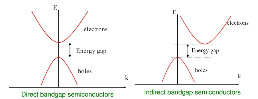
With this approximation, the matrix element simplifies to a term involving the momentum operator acting on the cell-periodic parts of the Bloch functions, ${\mathbf{p}}_{cv}(\mathbf{k})=⟨u_{c,\mathbf{k}}|\hat{\mathbf{p}}|u_{v,\mathbf{k}}⟩$.

Step 2: Summing Over All States & The Joint Density of States

Fermi's rule gives the rate for one transition. To find the total absorption rate per unit volume, $R_{up}$, we must sum over all possible initial states (all occupied $\mathbf{k}$ states in the valence band) and all possible final states (all empty $\mathbf{k}$ states in the conduction band).

Assuming the valence band is full ($f_v(\mathbf{k})=1$) and the conduction band is empty ($f_c(\mathbf{k})=0$), the sum becomes an integral over the Brillouin Zone:

$$R_{up}\propto {\int }_{BZ}{d}^{3}k|⟨{\psi }_c|{\hat{H}}^{\prime }|{\psi }_v⟩{|}^2\delta (E_c(\mathbf{k})-E_v(\mathbf{k})-\hslash \omega )$$

This integral introduces a crucial concept. The term ${\int }_{BZ}{d}^{3}k\delta (E_c(\mathbf{k})-E_v(\mathbf{k})-\hslash \omega )$ counts the number of pairs of states, one in the conduction band and one in the valence band at the same $\mathbf{k}$, that are separated by a specific energy $\hslash \omega$. This is the joint density of states (JDOS).

To evaluate this, we assume parabolic bands near the band edge, where most fundamental absorption occurs:

• $E_c(\mathbf{k})\approx E_g+\frac{{\hslash }^2{k}^2}{2m_e^{\ast }}$
• $E_v(\mathbf{k})\approx -\frac{{\hslash }^2{k}^2}{2m_h^{\ast }}$

The energy difference is $E_{cv}(\mathbf{k})=E_c(\mathbf{k})-E_v(\mathbf{k})=E_g+\frac{{\hslash }^2{k}^2}{2\mu }$, where $\mu =(1/m_e^{\ast }+1/m_h^{\ast }{)}^{-1}$ is the reduced effective mass of the electron-hole pair.

The JDOS can then be calculated, and it has a familiar form:

$$g_{joint}(\hslash \omega )=\frac{1}{2{\pi }^2}{\left(\frac{2\mu }{{\hslash }^2}\right)}^{3/2}\sqrt{\hslash \omega -E_g}$$

This $\sqrt{\hslash \omega -E_g}$ dependence is the key signature of a direct bandgap semiconductor.

Step 3: From Transition Rate to the Absorption Coefficient

The absorption coefficient $\alpha (\omega )$ is defined as the fraction of power absorbed per unit length. It relates the total energy absorbed per unit volume per second ($R_{up}\hslash \omega$) to the intensity of the incident light ($I$):

$$\alpha (\omega )=\frac{R_{up}\hslash \omega }{I}$$

By combining the results for the transition rate, the matrix element, and the joint density of states, and relating the vector potential $A_0$ to the intensity $I$, we arrive at the final expression.

The complete derivation is laid out in the following sections of the Cornell notes.

After working through the algebra, the absorption coefficient for a direct bandgap semiconductor is found to be:

$$\alpha (\omega )=C\frac{|{\mathbf{p}}_{cv}{|}^2}{\hslash \omega }\sqrt{\hslash \omega -E_g}$$

where $C$ is a collection of physical constants, and ${\mathbf{p}}_{cv}$ is the momentum matrix element, which is typically assumed to be roughly constant near the band edge. This equation tells us two crucial things:

1. Absorption is zero for photon energies below the bandgap ($\hslash \omega <E_g$).
2. Above the bandgap, absorption turns on and increases in proportion to $\sqrt{\hslash \omega -E_g}$.

4. Experimental Signatures and Analysis

This characteristic square-root dependence is a powerful tool used experimentally to identify direct bandgap materials and measure their bandgaps.

As the video shows, the agreement between our simple theory and experimental data for materials like Gallium Arsenide (GaAs) is remarkable. The sharp rise in absorption right above the bandgap energy is a clear fingerprint of a direct-gap material.

A common method for analyzing experimental data is to construct a Tauc plot. Based on our derived formula, if we plot $(\alpha \hslash \omega {)}^2$ versus photon energy $\hslash \omega$, we should get a straight line for a direct-gap material. Extrapolating this line to the energy axis gives a precise value for the bandgap $E_g$.

$$(\alpha \hslash \omega {)}^2\propto |{\mathbf{p}}_{cv}{|}^4(\hslash \omega -E_g)$$

Test your understanding!

The image below shows the absorption coefficient vs. wavelength for several semiconductors.

Based on the shape of their absorption curves, identify which of the unknown semiconductors (A, B, C) are likely to have a direct bandgap and which have an indirect bandgap. Briefly justify your answer.

Show answer

• Semiconductors A and C are likely direct bandgap materials. Their absorption coefficient $\alpha$ rises very sharply (by orders of magnitude over a short wavelength range) once the photon energy exceeds the bandgap energy (i.e., once the wavelength drops below the bandgap wavelength). This steep onset is characteristic of efficient, vertical, k-conserving transitions.
• Semiconductor B is likely an indirect bandgap material, similar to GaP shown in the plot. Its absorption coefficient rises much more gradually. This is because the absorption process near the band edge is less efficient, requiring the assistance of a phonon to conserve crystal momentum.

Conclusion

Today we have built a quantum mechanical model for the primary optical absorption mechanism in semiconductors. By applying Fermi's Golden Rule and the properties of Bloch electrons, we have derived the absorption coefficient and understood its direct link to the material's band structure.

Key Takeaways:

• Optical absorption in semiconductors is governed by interband transitions of electrons from the valence to the conduction band.
• The calculation is based on Fermi's Golden Rule, which requires the light-matter interaction Hamiltonian (${\hat{H}}^{\prime }\approx \frac{e}{m_0}\mathbf{A}\cdot \hat{\mathbf{p}}$) and the electronic wavefunctions (Bloch states).
• The dipole approximation leads to the crucial selection rule of vertical transitions (${\mathbf{k}}_c\approx {\mathbf{k}}_v$), explaining why direct bandgap materials are efficient absorbers.
• The absorption coefficient $\alpha (\omega )$ for a direct bandgap material is proportional to $\frac{1}{\omega }\sqrt{\hslash \omega -E_g}$.
• This theoretical dependence allows for experimental determination of bandgaps and the identification of direct vs. indirect gap materials via absorption spectroscopy and Tauc plots.

Preview of the Next Lesson

We have now modeled the dielectric response from both free carriers (Drude model) and interband transitions. These two processes determine the absorption and reflection of a material. However, the dielectric function's real (${ϵ}_1$) and imaginary (${ϵ}_2$) parts are not independent. In the next lesson, we will explore the profound connection between them by applying the Kramers-Kronig relations. This will allow us to determine a material's full optical response (e.g., its refractive index) just by measuring its absorption spectrum.