Single Training Step Implementation

Hello! Welcome to the next lesson in our journey into deep learning with PyTorch.

In our previous lesson, we assembled the essential components for training: a model defined with nn.Module, a loss function like nn.CrossEntropyLoss to measure error, and an optimizer like torch.optim.AdamW to drive the learning process. You now have the "what" (the model) and the "how" (the optimizer and loss function).

Today, we'll put these pieces into motion. This lesson is dedicated to implementing the most critical part of the entire deep learning process: a single training step. This is the fundamental engine that powers all model training. Our goal is to implement the sequence for a single training step: zero gradients, forward pass, compute loss, backward pass, and weight update. By the end, you'll understand the exact sequence of commands that makes a neural network learn from data.

The Five Steps of a Training Iteration

At its core, training a neural network is an iterative process. We show the model a small batch of data, calculate how wrong its predictions are, and then nudge its parameters in the right direction to make it a little less wrong. This cycle, when repeated thousands of times, is what we call "training."

A single one of these cycles, or a "training step," consists of five key actions performed in a specific order:

1. Forward Pass: The model makes a prediction based on the input data.
2. Compute Loss: The loss function compares the model's prediction to the true labels and calculates a single loss value.
3. Backward Pass: PyTorch's autograd engine calculates the gradient of the loss with respect to every learnable parameter in the model. This tells us the direction to move each parameter to reduce the loss.
4. Update Weights: The optimizer uses the calculated gradients to "step" the model's parameters in the direction that minimizes the loss.
5. Zero Gradients: The gradients are reset to zero to prevent them from accumulating in the next iteration.

This sequence is universal across virtually all deep learning training procedures.

From First Principles to Professional Practice

To understand this process deeply, we'll first see it built from the ground up, and then see how PyTorch's tools make it clean and efficient. The following video provides a brilliant walkthrough of this entire process.

Dissecting the Training Step in PyTorch

As you saw in the video, while the "from scratch" implementation is insightful, the professional PyTorch approach is much cleaner. It revolves around the three objects you've already prepared: your model, your loss function, and your optimizer.

Let's summarize the professional sequence with the corresponding PyTorch commands.

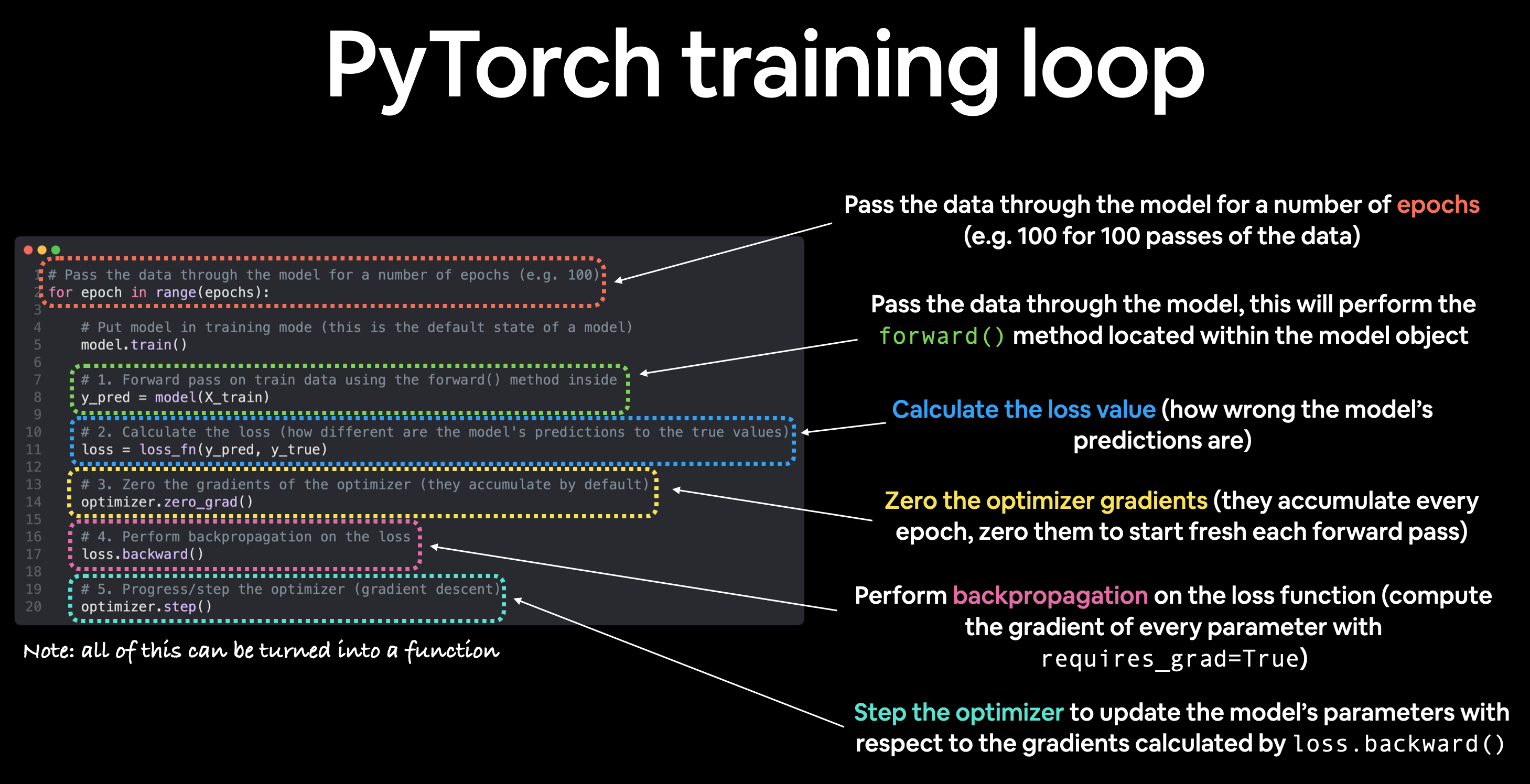
Here is a breakdown of the core logic:

1. Forward Pass: y_pred = model(X_batch)

   • You pass a batch of input data (X_batch) to your model instance.
   • PyTorch calls the forward() method you defined, and the model returns its raw predictions (logits).

2. Compute Loss: loss = loss_fn(y_pred, y_batch)

   • You pass the model's predictions and the corresponding true labels (y_batch) to your loss function instance.
   • It returns a single tensor containing the loss value for the batch. This loss tensor keeps track of the entire computation graph needed for backpropagation.

3. Zero Gradients: optimizer.zero_grad()

   • This is a crucial housekeeping step. By default, PyTorch accumulates gradients every time .backward() is called. We must clear the old gradients from the previous step before calculating new ones. The optimizer holds references to all the model's parameters, so it provides a convenient method to do this for all of them at once.

4. Backward Pass: loss.backward()

   • This is where the magic happens. You call .backward() on the loss tensor.
   • PyTorch's autograd engine traverses the computation graph backward (from the loss all the way to the input) and computes the gradient ($\frac{\partial \text{loss}}{\partial \theta }$) for every parameter $\theta$ that has requires_grad=True. These gradients are then stored in the .grad attribute of each respective parameter tensor.

5. Weight Update: optimizer.step()

   • Now that the gradients are computed and stored in each parameter's .grad attribute, we call optimizer.step().
   • The optimizer iterates through all the parameters it was given during initialization and updates them using its specific update rule. For SGD, it would be theta -= learning_rate * theta.grad. For AdamW, it's a more complex but similar idea. This is the step where the model actually learns.

This sequence—zero gradients, forward, loss, backward, step—is the atomic unit of training.

The following reading provides a wonderfully concise function, make_train_step, that encapsulates this entire logic.

A Complete Example

Let's bring this all together with the model from our last lesson. We'll create some dummy data and perform exactly one training step.

import torch
import torch.nn as nn




# --- Setup from previous lessons ---




# 1. Define the model
class SimpleMLP(nn.Module):
    def __init__(self, input_size, hidden_size, num_classes):
        super().__init__()
        self.network = nn.Sequential(
            nn.Linear(input_size, hidden_size),
            nn.ReLU(),
            nn.Linear(hidden_size, num_classes)
        )

    def forward(self, x):
        return self.network(x)




# 2. Instantiate model, loss, and optimizer
input_dim = 784
hidden_dim = 512
class_count = 10
learning_rate = 0.001

model = SimpleMLP(input_size=input_dim, hidden_size=hidden_dim, num_classes=class_count)
loss_fn = nn.CrossEntropyLoss()
optimizer = torch.optim.AdamW(model.parameters(), lr=learning_rate)




# --- Create dummy data for one batch ---
batch_size = 4
X_batch = torch.randn(batch_size, input_dim)  # 4 samples, 784 features each
y_batch = torch.randint(0, class_count, (batch_size,)) # 4 labels, with values from 0-9

print(f"Original weight of first layer: {model.network[0].weight.data[0, :5]}")
print("--- Starting One Training Step ---")




# ----- THE TRAINING STEP SEQUENCE -----




# Step 1: Forward Pass
y_pred_logits = model(X_batch)
print(f"Prediction logits shape: {y_pred_logits.shape}")




# Step 2: Compute Loss
loss = loss_fn(y_pred_logits, y_batch)
print(f"Calculated Loss: {loss.item():.4f}")




# Step 3: Zero Gradients
optimizer.zero_grad()




# Step 4: Backward Pass (Compute Gradients)
loss.backward()



# Gradients are now stored in `parameter.grad` for every parameter




# Step 5: Update Weights
optimizer.step()




# --- End of Training Step ---
print("--- Finished One Training Step ---")
print(f"Updated weight of first layer:   {model.network[0].weight.data[0, :5]}")

If you run this code, you will see that the Original weight and Updated weight are different. The optimizer.step() call has successfully modified the model's parameters based on the computed loss and gradients. You have made the model learn!

Conclusion

In this lesson, you've mastered the heart of the PyTorch training process. While it may seem like a lot of steps, the sequence quickly becomes second nature.

Key Takeaways:

• A training step is a five-action sequence: Forward Pass -> Compute Loss -> Zero Gradients -> Backward Pass -> Weight Update.
• In PyTorch, this translates to calling model(), loss_fn(), optimizer.zero_grad(), loss.backward(), and optimizer.step().
• The three lines optimizer.zero_grad(), loss.backward(), and optimizer.step() form the core "engine" of learning in most PyTorch training loops.
• Each component (model, loss_fn, optimizer) has a distinct and separate role in this process.

You now have all the tools to train a model on a single batch of data. But deep learning models are trained on thousands of batches over many cycles, or "epochs." Furthermore, for large models, these computations can be very slow on a CPU.

In our next lesson, we will address this by learning how to move our tensors and models to a GPU to accelerate training, setting the stage for training on full datasets.