Recommended resources
The freely available resources this lesson will direct you to.
Hello. Earlier modules developed the physics of radiative forcing and examined how temperature records are constructed. This module asks a different question: how can we distinguish the causes of an observed change? Today you will formulate optimal fingerprinting as a multiple regression, identify precisely what its observations and predictors are, and see why accounting for natural variability changes the fit.
Your econometrics background is useful here. The algebra is familiar, but the design of the regressors is unusual: they are model-simulated climate responses, not raw measurements of emissions or solar activity.
From a temperature trend to an attribution question
Suppose an observed temperature record warms. A trend establishes that change occurred; by itself, it does not say what caused it. Several influences may act at once. Greenhouse gases tend to warm the climate, anthropogenic aerosols can offset some warming, and changes in solar output or volcanic activity can also affect temperature. Meanwhile, internal variability—fluctuations arising within the climate system, such as ENSO—changes temperatures without requiring a change in external forcing.
Optimal fingerprinting asks whether the pattern of observations can be represented as a combination of expected responses to these external influences, allowing for internal variability. “Pattern” can mean more than a single global-mean time series: it may contain temperatures from multiple places, decades, or atmospheric levels. That extra structure can help distinguish influences whose global means look similar.
The distinction between two kinds of natural change matters throughout this lesson:
- Naturally forced change is a response to an external influence such as solar variability or volcanic eruptions.
- Internal variability is the climate system’s unforced fluctuation. In the regression, it is principally part of the noise, not another forcing fingerprint.
The following presentation gives a compact account of what enters the regression and how the data are prepared.
Read the selected slides from Francis Zwiers’s Detection and attribution presentation to see how a climate attribution question becomes a regression with observed temperatures, simulated signals, scaling factors, and residuals.
Start on the slide introducing Y as observations, X as expected changes, and regression coefficients as scaling factors. Read the regression rationale. Then find the slides headed “Applying the simple OLS form,” especially “Observations Y” and “Signals Xi, i=1, …, s.” Read the observations example and the signal construction. Finally, under “Review of Basic Procedure,” read the data-preparation steps. Focus on why simulated signals must be processed on the same spatial and temporal footing as observations.
The multiple regression model
Let be a column vector containing observed temperature anomalies. An entry might represent one region in one decade; the entries can also describe vertical atmospheric layers or another consistently defined set of observations. Stack the corresponding model-simulated responses into columns of a matrix . The basic model is
Here each is an -entry fingerprint: the expected temperature-response pattern associated with the specified forcing. The vector contains unknown scaling factors, and contains departures from the scaled patterns, principally internal variability. If has three columns, its dimensions are , while is . Some studies use a two-column specification, with one combined anthropogenic fingerprint and one naturally forced fingerprint.
It is worth being exact about the predictors. is not an atmospheric CO₂ concentration series. It is the simulated temperature response to greenhouse-gas forcing over the chosen times and places. Similarly, is not a raw solar-irradiance series: it represents the simulated response to the natural forcings included in that experiment, commonly solar and volcanic influences. Ensemble averaging helps estimate each forced response while reducing the simulation’s particular realization of internal variability.
The observations and signals need compatible units, reference periods, spatial coverage, and time averaging. If an observational grid cell is missing, comparing it to a complete model grid without matching the coverage could create an apparent pattern difference that has nothing to do with the forcing. Anomalies are commonly defined relative to a shared reference period, so the basic fingerprint regression is often written without a separate intercept.
A deliberately noise-free example shows what a scaling factor does. Suppose three entries of the vectors, all expressed as temperature anomalies in °C, are:
| Entry | Greenhouse-gas signal | Natural-forcing signal | Observation |
|---|---|---|---|
| 1 | 0.10 | 0.10 | 0.15 |
| 2 | 0.20 | 0.00 | 0.20 |
| 3 | 0.30 | −0.10 | 0.25 |
These observations equal one times the greenhouse-gas signal plus 0.5 times the natural-forcing signal. Thus the two fitted scaling factors would be and . The factors multiply whole response patterns, not individual data points independently. Real observations do not line up exactly: the residual vector records what remains after fitting.
Why the fit is “optimal”
Ordinary least squares minimizes the squared length of the residual vector, . But climate residuals are not equally variable or independent across entries. For example, temperatures in neighboring regions can fluctuate together; some spatial patterns of internal variability are much stronger than others. Treating every direction in the data as equally informative would discard that knowledge.
Let describe the covariance of internal variability. In the idealized case where the fingerprint columns are treated as known and the covariance is invertible, generalized least squares minimizes
and gives
This is the statistical core of the “optimal” in optimal fingerprinting. Relative to directions in which internal variability is large, the fit gives more weight to directions where a forced signal stands out against that variability. It does not mean the method eliminates noise or guarantees a correct attribution. Estimating itself is demanding; studies commonly use long model control simulations without changing external forcing and often reduce the data dimension before fitting.
For the geometric intuition and the formal model, read the two short parts of the IPCC chapter below. Its terminology uses for the signal matrix and for scaling factors, in place of and .
[PDF] Detection of Climate Change and Attribution of Causes
Read Box 12.1 and the opening of Appendix 12.1 of the IPCC’s Detection of Climate Change and Attribution of Causes. The box explains the signal-to-noise idea; the appendix states the regression and covariance-weighted estimator.
In Box 12.1, read the two-mode example. Track why a component of a signal can be more detectable even when its projected magnitude is smaller. Then go to “Appendix 12.1: Optimal Detection is Regression.” Read its opening through equations (A12.1.1)–(A12.1.3), using the field description to identify the observations and simulated signals, and the estimation discussion to connect the equations to the weighting intuition. The PDF’s equations are clearer on the page than in extracted text.
Reading scaling factors as evidence
A fitted near means the magnitude of the observed greenhouse-gas-associated pattern is consistent with the model-simulated pattern within the fitted specification. A factor above means that pattern needs to be amplified to fit; one below means it needs to be reduced. Whether either difference is meaningful depends on uncertainty.
Two questions should not be conflated:
- Detection: Is a scaling factor distinguishable from zero, given its uncertainty? If so, that fingerprint has been detected under the model’s assumptions.
- Consistency: Is the scaling factor compatible with , the simulated response magnitude? A factor need not be exactly for the model and observations to be consistent.
A scaling factor is also not a temperature contribution in °C. To estimate a forcing’s attributable contribution over a specified region and period, scale its simulated response and then calculate the change of interest from that scaled response. A negative aerosol temperature contribution, for instance, can arise from a positive aerosol scaling factor multiplying a simulated cooling pattern.
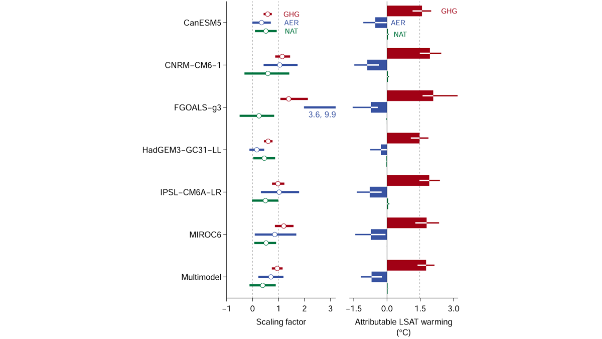
Notice the conceptual distinction between the panels before comparing bar lengths. The plotted analysis associates greenhouse gases with warming and aerosols with an offsetting cooling contribution. The natural-forcing contribution shown is small. That finding concerns this analysis and its land-temperature measure; the figure alone does not establish the contribution of every possible influence to every climate variable.
What the regression can—and cannot—separate
The regression’s explanatory power depends partly on how distinct its columns are. If two simulated fingerprints are nearly proportional across the chosen observations, a change in one scaling factor can be offset by a change in the other. The combined response may be well determined while the individual contributions are not. This is the familiar multicollinearity problem, with an important physical consequence: a fit to warming is not necessarily a clean separation of its causes. Using spatial or temporal structure can improve separation when the influences have different patterns.
There are further checks behind a credible result. The estimated residuals should be plausible relative to independently assessed internal variability. The forced fingerprints must be sufficiently realistic, and a finite ensemble does not yield a perfectly known predictor matrix. Observational errors or omitted responses can also affect the fit. These considerations explain why attribution is more than finding statistically significant coefficients in a convenient regression.
The central formulation remains straightforward: observed climate changes are the dependent vector; simulated responses to specified anthropogenic and natural forcings are the independent columns; scaling factors are estimated while accounting for internal variability. What makes the exercise scientific attribution rather than pattern matching is the physical construction of those columns and the scrutiny of whether the fitted model adequately explains the observations.
Key takeaways
Optimal fingerprinting expresses an observed temperature pattern as a linear combination of simulated forced-response patterns plus residual variability. Generalized least squares uses an estimate of internal-variability covariance to emphasize information with a stronger signal-to-noise ratio. Scaling factors describe how strongly each simulated pattern appears in the observations; they are distinct from the resulting temperature contributions, and their interpretation depends on uncertainty and model adequacy.
The next lesson turns from estimating those signals to the IPCC’s formal language for evaluating and communicating uncertainty in attribution statements.