Recommended resources
The freely available resources this lesson will direct you to.
Hello. In the previous lesson, you distinguished a climate projection from a weather forecast and saw why model skill must be judged against the claim a model makes. That principle becomes especially important when a model has been tuned: if developers used an observation to adjust a model, agreement with that same observation is not an independent test.
This is the final lesson of the course. We will examine why tuning is often necessary, how it can conceal errors, and what evidence can still establish credibility. The aim is neither to dismiss models because they use observations nor to treat a good historical fit as sufficient proof of future accuracy.
Why a physics-based model still needs tuning
A global climate model cannot calculate every turbulent eddy, cloud droplet and exchange at the land surface. It resolves motions on a finite grid; processes smaller than that grid need approximate representations called parameterizations. These representations are constrained by physics and observations, but some of their parameter values cannot be determined precisely from first principles.
Read the opening discussion in The Art and Science of Climate Model Tuning, by Hourdin and colleagues. It separates choices about what a model represents from choices about the values used within that representation.
Read this to distinguish a physical model, an approximate representation of an unresolved process, and calibration of that representation.
In “DEFINITION OF CLIMATE MODEL TUNING,” begin with the paragraph on motions resolved by the model grid. Read the discussion of parameterizations and computing trade-offs. Then, in the same section, read the definition of tuning. Focus on why selecting a parameter value is different from—but cannot be wholly separated from—choosing the model's structure.
In the narrow sense used here, tuning is selecting uncertain parameter values so that specified model outputs agree acceptably with observations or other defensible targets. It is not a licence to alter conservation of energy whenever a result is inconvenient. Nor is it peculiar to climate science: estimating uncertain quantities is a normal part of building a quantitative model.
Your earlier one-layer energy-balance model illustrates the distinction. Its assumption that the atmosphere absorbs all surface infrared radiation is a structural simplification. Replacing that assumption with a more realistic treatment changes the model formulation. Choosing an uncertain cloud-process parameter within a particular formulation is calibration. Either decision can change the simulated climate, but they present different scientific questions.
Greater complexity can improve fidelity by representing processes that a simpler model omits. It also brings additional parameters and interactions that must be constrained, while finer resolution makes each simulation more expensive. Given finite computing time, increasing resolution or adding processes can reduce the number or length of simulations available for testing parameter choices. More detail is valuable when it improves the representation of relevant processes, not simply because it makes a model larger.
The genuine risk: a good fit for the wrong reason
A model might match a chosen target while misrepresenting the mechanisms that produce it. In statistical terms, calibration and evaluation cease to be cleanly separated when the same information influences both.
Suppose developers choose parameters to make simulated diagnostics close to observed diagnostics . A schematic calibration criterion is
where expresses how discrepancies are weighted. Minimizing can be useful, but the answer depends on which diagnostics enter and how uncertainty and model error are represented. A low score does not establish that omitted processes are correct.
The authors discuss both systematic calibration and its failure modes:
Continue with the article to see why making tuning more systematic does not remove scientific judgment or the possibility of overfitting.
In “APPLYING OBJECTIVE METHODS,” read the opening discussion of objective methods. Then find the paragraph beginning “A principal challenge for automatic tuning methods” and read the account of overtuning. Focus on the difference between improving a selected score and improving the model's representation of the world.
The danger is not limited to an optimizer with too many adjustable parameters. A developer tuning by hand can also compensate for one error with another. Conversely, an objective function makes trade-offs explicit but does not make their selection objective: someone still decides which observations matter and how much weight they receive.
Overfitting has a particularly important interpretation here. A parameter choice may capture features of one observed period that arose partly from internal variability rather than from the process the parameter is meant to represent. Or it may improve global mean temperature while worsening a cloud property, a regional pattern or a response to changed forcing. A better-looking curve can therefore be a poorer explanation.
How two models can match historical warming yet disagree about the future
Consider a deliberately simplified global energy-balance approximation:
where is net historical radiative forcing, is the rate of heat uptake—principally by the ocean—and is a positive restoring-feedback parameter, measured in watts per square metre per kelvin. This is an illustration, not a reconstruction of the historical climate.
Imagine two models with the following hypothetical values, all forcing and heat-uptake quantities in watts per square metre:
| Greenhouse-gas forcing | Aerosol forcing | |||
|---|---|---|---|---|
| Model A | ||||
| Model B |
Model A gives K. Model B also gives K. Both match the same hypothetical historical warming. But Model B combines stronger aerosol cooling with a stronger temperature response per unit net forcing.
If we instead compare their simplified equilibrium responses to the same CO₂-doubling forcing of approximately watts per square metre, the heat-uptake term has fallen to zero at equilibrium. Their respective estimates become K and K. Historical temperature agreement alone could not distinguish them.
Real forcing, ocean uptake and feedbacks are more complicated than these fixed numbers. The example establishes a narrower logical point: a historical global-temperature fit does not uniquely identify the combination of aerosol effects and climate sensitivity that generated it.
This issue is explicitly debated in The Art and Science of Climate Model Tuning:
Read the article's discussion of whether observed historical warming should serve as a tuning target, an evaluation test, or partly both.
In “TUNING TO TWENTIETH-CENTURY WARMING?”, start with the opening problem. Later in that section, read the three uncertainties affecting a historical-warming match. Finish with the closing discussion of differing development practices. The intervening figure and case study are optional; the key question is how knowing the historical result changes its status as a test.
There is no need to claim that every model was deliberately adjusted to reproduce twentieth-century warming. Developers may use different practices, and even a target not explicitly included in a calibration criterion can influence development decisions when its observed value is well known. Equally, the existence of that risk does not show that a particular future projection is wrong. It tells us to ask what was adjusted, using which evidence, and what remains to be tested independently.
Read parameter sweeps as evidence of uncertainty, not proof of failure
The figure below shows how varying individual model parameters changes simulated top-of-atmosphere radiation and cloud cover. The horizontal bands provide observational reference ranges.
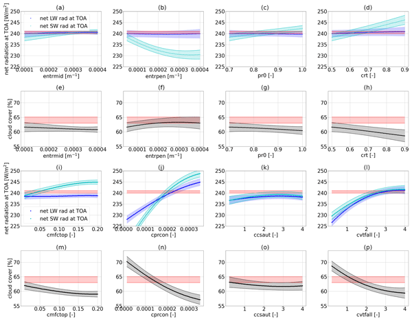
For example, compare the paired panels labelled (j) and (n): as the parameter on their common horizontal axis changes, both radiation diagnostics and cloud cover change substantially. One parameter may improve agreement with one observed quantity while shifting another. The figure is thus more informative than a single “best-fit” score: it shows why several relevant targets need to be considered together.
It also has limits. Each displayed sweep changes a parameter over a specified range; it does not, by itself, establish what happens when several parameters change together or whether a parameter value is physically plausible. And agreement with the plotted reference bands would be less compelling as an independent test if those same references had been used to select the parameters.
A review of model benchmarking makes both points concrete: different tunings can yield similarly plausible broad climate diagnostics while differing in regional behaviour and climate sensitivity, and overfitting remains a reason to devise fresh tests.
Systematic Benchmarking of Climate Models
Read these short passages from Hassler and colleagues to connect tuning choices with the limits of model evaluation.
In the discussion on printed p. 10, locate the paragraph beginning “Once a model is developed to the point of producing climate simulations” and read the tuning example, including the different results obtained from plausible tunings. Later in the review, find the paragraph beginning “Even as software tools are developed” and read why new observational tests matter. Then find the paragraph beginning “Despite efforts to mitigate overfitting” and read its concluding caution. Focus on what a successful fit to selected targets leaves unresolved.
What would make the assessment fair?
The categorical argument—“models are tuned, therefore they are unreliable”—does not follow. Calibration is necessary when important processes cannot be resolved or their parameters measured exactly. The opposite categorical argument—“models match past warming, therefore their projections are reliable”—does not follow either.
A stronger assessment starts with the intended use of a model. Confidence in a global, multi-decade temperature response is not automatically confidence in local rainfall or cloud cover. For the quantity at issue, ask:
- What information influenced development? Include explicit calibration targets and known observations that may have guided model selection.
- Are the chosen parameter values and processes defensible? A match obtained with implausible settings is a warning, not an achievement.
- Does the model reproduce other relevant evidence? Process-level observations, variables not used as targets, different climate conditions and subsequently observed behaviour can reveal compensating errors. None is automatically a perfect holdout: development choices can draw on shared information.
- How sensitive is the conclusion to structural and parameter choices? Alternative plausible configurations may match the historical record yet produce different future responses. Agreement across models is useful, but related models are not necessarily independent pieces of evidence.
These checks connect to the earlier lessons on hindcasting and ensembles. Testing a model against historical data remains informative, provided you distinguish agreement on targets used to develop it from performance on additional, relevant tests. No single score certifies a model for every purpose.
Conclusion
Tuning is parameter estimation within an imperfect physical model, not evidence by itself of scientific misconduct or model failure. It is needed because finite-resolution models use approximate representations of unresolved processes. Its real hazards are overfitting, compensating errors and mistaking agreement with a development target for independent validation. Greater complexity can address missing physics, but also increases computational and calibration demands; greater fidelity must be demonstrated rather than assumed.
The most defensible judgment is therefore specific: identify the projected quantity, disclose how the model was tuned, and look for physically credible performance across tests capable of exposing a good fit for the wrong reason. That completes the course’s progression from basic climate physics through evidence, attribution and the critical evaluation of climate models.