GCM Architecture: Resolved vs. Parameterized Processes

Hello. In the previous lesson, simulations driven only by natural influences failed to reproduce the broad pattern of recent warming. To judge what that comparison tells us, we need to look inside a climate model. What does it calculate from physical laws, and where must it use approximations?

This lesson builds a working picture of a general circulation model (GCM): a three-dimensional grid, equations for large-scale motion, representations of processes too small or otherwise impractical to calculate directly, and exchanges between the atmosphere and the rest of the climate system. The distinction between resolved and parameterized processes is central—but it is not a distinction between “physics” and “guesswork.”

A planet represented by cells

Imagine dividing the atmosphere into horizontal grid boxes and stacking layers above each one. At each time step, an atmospheric model tracks quantities such as temperature, pressure, wind and water vapour in those cells. An ocean model likewise tracks quantities including temperature, salinity and currents. The governing equations express conservation of mass, momentum and energy; numerical methods approximate their solutions on the grid.

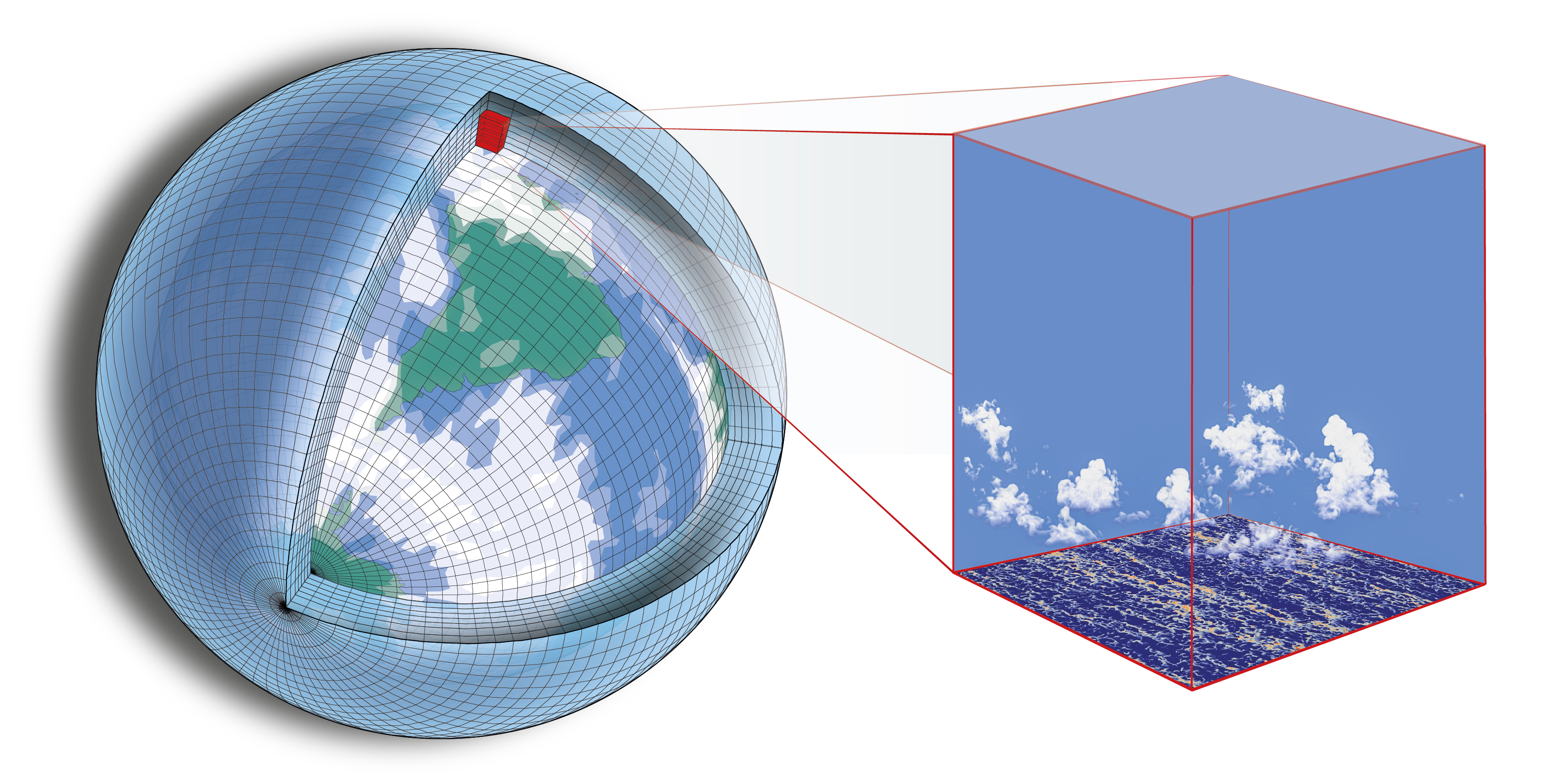
Watch two short passages from The Economist’s How scientists calculate climate change. The first shows the grid; the second introduces the problem posed by clouds.

“Resolved” means that variations across multiple grid cells can be represented in the model’s calculated state. A broad pressure system, for example, can appear as a pattern of pressures and winds across many cells. The model calculates how that pattern develops; a modeller does not draw each future pressure system into it.

A feature is not accurately resolved merely because it is as wide as one cell. Its shape, movement and interactions generally need several cells to be represented well. Thus grid spacing is not the same as effective resolution. Finer spacing can reveal more detail, but it also increases computational cost—particularly when simulations must cover many decades.

A GCM is consequently neither a collection of hand-drawn climate patterns nor a microscopic simulation of every parcel of air. It is a numerical calculation at a chosen scale. That choice determines which effects need another treatment.

Where the dynamical core ends

The dynamical core is the part of an atmospheric GCM that advances resolved fluid motion and related thermodynamic fields on the grid. It handles such tasks as the transport of air, heat and moisture by resolved winds. Alongside it sits a parameterization suite, whose calculations supply effects that the dynamical core does not explicitly represent.

The following tutorial slides state that division particularly clearly. They are more technical than the video, so focus on the architecture rather than the named numerical schemes.

There are two reasons a process might sit outside the dynamical core. It may occur mainly below the grid’s resolvable scale, as much turbulence and individual convective updrafts do. Or it may require a different calculation from the equations of fluid motion. Radiative transfer is an example: models calculate how radiation is absorbed, emitted and scattered through atmospheric columns, commonly using a specialised radiation scheme. Calling that scheme a parameterization does not mean that sunlight or infrared radiation is merely guessed.

A compact way to think about one model variable is:

The other schemes use information available from the grid—such as temperature, humidity and wind—and return changes to the grid-scale state. Those changes must be reconciled with physical constraints, including conservation of mass and energy. The precise numerical division differs among models, but the architectural idea is widely shared.

Why averaging creates a missing term

Your statistics background offers a precise way to see why unresolved motions cannot simply be ignored. Let $w$ denote vertical air velocity and $q$ the amount of water vapour per unit mass of air. Their product contributes to vertical moisture transport. If a bar denotes a cell-scale average and a prime denotes a departure from that average, then

The first term describes transport associated with the resolved mean flow. The second captures covariance within the cell. Even when mean vertical velocity is near zero, small rising regions can carry moist air while sinking regions carry drier air, producing a non-zero moisture transport. Keeping only the cell means would miss it.

A turbulence parameterization estimates the missing transport from quantities the model does track. One simplified approach relates turbulent moisture transport to the vertical gradient of mean humidity:

where $K_q$ represents the strength of turbulent mixing. This is an illustrative closure: an approximation that expresses an unresolved quantity in terms of resolved ones. It is not a universal formula for every atmosphere or a description of how clouds themselves are calculated.

For a closer look, the next video connects grid averaging to missing transport and then applies the scale problem to convection and clouds.

Clouds: present in the model, not necessarily resolved by it

Consider a hypothetical horizontal cell 100 kilometres wide containing a convective cloud system 10 kilometres wide. The cell’s average temperature and humidity cannot describe the rising plume, its surrounding sinking air, and all their exchanges separately. Yet those exchanges move heat and moisture, produce precipitation and alter radiation. Omitting them would not leave a more “purely physical” model; it would leave out consequential physics.

Clouds reveal a further problem with averages: the effect of an average state is not necessarily the average effect of its varied parts. Suppose, purely as an illustration, that two equal areas at the same temperature have relative humidities of 100% and 40%. Their mean is 70%, but the mean conceals an area at saturation where cloud formation may occur. A scheme that treated the whole box as uniformly 70% humid could miss that possibility. Real cloud schemes use more information and more sophisticated assumptions than this toy example, but they face the same underlying issue.

Different schemes therefore estimate related quantities: whether convection occurs and how it transports heat and moisture; how much of a cell contains cloud; and cloud properties relevant to precipitation and radiation. These estimates interact. Clouds affect the climate both by reflecting incoming sunlight and by absorbing and emitting infrared radiation. Their net effect depends in part on cloud amount, altitude and optical properties—features that are difficult to infer perfectly from cell averages.

Parameterized does not mean physically arbitrary. A cloud scheme is intended to embody physical understanding and is assessed against observations and more detailed simulations. But it does introduce approximations, and different defensible schemes can yield different climate responses. Nor does a finer grid automatically eliminate the problem: some larger cloud systems become better resolved, while smaller turbulent motions and cloud-particle processes remain below grid scale. As resolution changes, the parameterizations may need to change too.

More than an atmosphere

For climate change, the atmosphere cannot sensibly be treated in isolation. It exchanges heat, water and momentum with the ocean; land affects evaporation and surface heating; snow and sea ice alter reflection of sunlight and exchange energy with their surroundings. In a coupled climate model, component models communicate these quantities at their shared boundaries as the simulation advances.

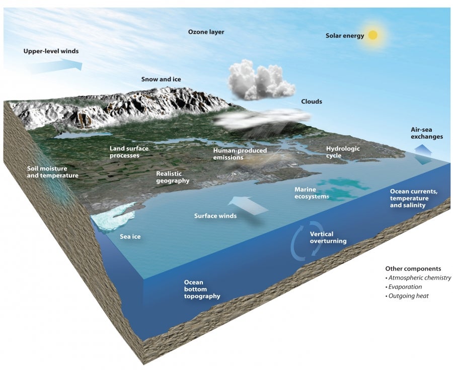
For example, an ocean component can calculate large-scale currents and heat transport on its own grid, while also representing smaller-scale mixing. At the surface, atmosphere and ocean components exchange calculated heat and water fluxes. Coupling matters because warming is not determined solely by what happens to air temperature: the ocean can take up heat and release it over time.

The scope of models varies. Some simulations prescribe atmospheric greenhouse-gas concentrations as inputs; more extensive Earth system models may also represent parts of the carbon cycle and other chemistry or biology. A useful architectural description is therefore not “one program calculates everything.” It is gridded component models, physical equations, parameterization schemes and exchanges between components, assembled for a particular scientific question.

What this architecture lets you judge

A GCM calculates large-scale evolution from physical equations on a finite grid. Its dynamical core represents resolvable motion; parameterization schemes supply the effects of unresolved processes and specialised processes, such as radiation, that lie outside the core. Clouds are a prominent example because their small-scale structure has large-scale consequences. Coupled components extend the calculation across atmosphere, ocean, land and ice.

This picture makes the earlier natural-only simulation comparison easier to interpret. Such a simulation is a physically structured test of how the modelled climate responds to specified influences, not a direct calculation of every cloud on Earth. Its credibility depends partly on how well the combined model represents the processes that matter. The next lesson examines how that credibility is tested against historical observations and other climate evidence, including what can—and cannot—be learned from multiple models.