Convolutional Layer Mechanics

Introduction

In our last lesson, we established the theoretical foundation of Convolutional Neural Networks, focusing on how the convolution operation and parameter sharing give rise to translation equivariance and enable the learning of spatial feature hierarchies. We noted that the convolution operation itself, depending on the filter size, alters the spatial dimensions of the feature maps.

Today, we will build directly on that knowledge by exploring the mechanisms that give us explicit control over these spatial dimensions. This lesson focuses on three fundamental components of a CNN architecture: padding, stride, and pooling layers. You will learn not only their mechanical function but also their strategic purpose in designing effective and efficient deep learning models for vision. Understanding these tools is essential for controlling information flow, managing computational complexity, and building a degree of invariance into the network.

Controlling Spatial Dimensions: Padding and Stride

In the previous lesson, you saw that convolving an input with a filter (e.g., a 3x3 filter on a 32x32 image) produces a slightly smaller output (e.g., 30x30). If we stack many such layers, the feature maps would shrink rapidly, causing two problems:

1. The spatial dimensions would diminish, possibly before we have extracted sufficiently high-level features.
2. Information at the borders of the original image would be progressively "washed away," as those pixels participate in far fewer convolutions than pixels at the center.

To manage this, we use two key hyperparameters in our convolutional layers: padding and stride.

Padding: Preserving Boundaries and Dimensions

Padding is the process of adding extra pixels, typically with a value of zero, around the borders of an input volume before the convolution.

The primary motivations for padding are:

• Preserving Spatial Size: By adding the right amount of padding, we can ensure the output feature map has the same width and height as the input. This is often called "same" padding and is a very common strategy. It simplifies network design, as we don't need to constantly track shrinking dimensions.
• Retaining Border Information: Padding allows the filter's receptive field to be centered on border pixels, ensuring they are treated more equally to interior pixels.

The following resource provides a clear introduction to padding and the formula for the resulting output size.

As the reading explains, if an input has width $W$, the filter has width $F$, the padding is $P$, and the stride is $S$, the output width is given by:

A common rule of thumb for "same" padding with a stride of $S=1$ is to set the padding $P=(F-1)/2$. For a 3x3 filter, we use $P=1$. For a 5x5 filter, we use $P=2$.

Stride: Downsampling and Efficiency

Stride defines the step size the filter takes as it slides across the input. In all our examples so far, we have implicitly used a stride of 1. By increasing the stride, say to 2, the filter skips every other pixel.

The primary motivations for using a stride greater than one are:

• Downsampling: It directly reduces the spatial dimensions of the output feature map, acting as a form of subsampling.
• Computational Efficiency: A larger stride means fewer convolution operations are performed, reducing the overall computational load.
• Increasing Receptive Field: Downsampling causes the effective receptive field of subsequent layers to grow more quickly with respect to the original input.

This interactive lecture segment provides an excellent walkthrough of how stride works and its effect on output size.

The image below visualizes four common scenarios involving different padding and stride settings.

For a deeper dive into the technical details and a classic real-world example, the CS231n notes are an invaluable resource.

Pooling Layers: Summarizing and Invariance

While a strided convolution effectively downsamples the feature maps, a more explicit and historically dominant method is the pooling layer. Pooling is a separate, non-parametric layer typically inserted between successive convolutional layers.

Its function is to progressively reduce the spatial size of the representation. This serves several purposes:

1. It further reduces the number of parameters and computational cost in the network.
2. It helps to control overfitting by providing a summarized, more abstract representation.
3. Critically, it introduces a degree of translation invariance.

Recall that convolution is translation equivariant: shifting the input shifts the output. A pooling operation, by summarizing a local neighborhood, can make the representation robust to small shifts of a feature within that neighborhood. For example, with 2x2 max pooling, as long as the most activated neuron remains within that 2x2 window, the output will be identical, regardless of its precise position.

The most common type of pooling is max pooling. It operates independently on each depth slice of the input volume. A window (e.g., 2x2) slides over the feature map, and at each position, only the maximum value within the window is passed to the output.

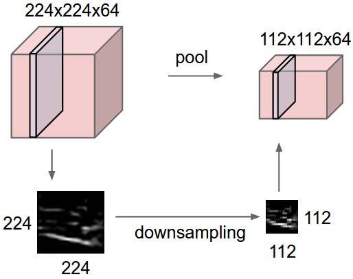
The following resource provides a thorough explanation of pooling layers.

To see pooling in action, this short video offers a clear, animated explanation.

Architectural Patterns

With these components, we can define a standard "block" in a typical CNN architecture: CONV -> RELU -> POOL. A common and effective design pattern is to use the layers for distinct purposes:

• Convolutional Layers: Use small filters (e.g., 3x3), a stride of 1, and "same" padding. Their role is to perform feature extraction, transforming the input depth-wise while preserving the spatial dimensions.
• Pooling Layers: Use a 2x2 filter with a stride of 2. Their role is exclusively to downsample the spatial dimensions, typically halving them.

This separation of concerns—feature learning in CONV layers, downsampling in POOL layers—makes designing and debugging architectures much more straightforward.

Conclusion

In this lesson, we have moved beyond the core convolution operation to understand the tools that shape the flow of information through a CNN. These hyperparameters and layers are not mere implementation details; they are fundamental design choices with significant theoretical and practical implications.

Here are your key takeaways:

• Padding adds a border of pixels to an input volume, primarily to preserve spatial dimensions across convolutional layers and ensure features at the image boundary are fully processed.
• Stride is the step size of the filter. A stride greater than 1 is a method of downsampling, reducing both the feature map size and the computational cost.
• Pooling Layers, most commonly implementing max pooling, serve as dedicated downsampling stages. They reduce dimensionality, control overfitting, and introduce a small degree of local translation invariance, a crucial property for robust recognition.
• A common architectural pattern involves using padded, stride-1 convolutions for feature learning and stride-2 pooling layers for spatial downsampling.

In our next lesson, we will pivot from architectures designed for spatial data to those designed for sequential data. You will be introduced to the Recurrent Neural Network (RNN), an architecture that processes information through time, opening the door to tasks in natural language processing, time-series analysis, and more.