Convolution and Parameter Sharing in CNNs

Introduction

In our last lesson, we explored the fascinating geometry of deep learning optimization, discovering that architectural choices, like the skip connections in ResNets, can fundamentally reshape the loss landscape to make training more tractable. This insight provides a perfect bridge to our next topic: exploring specialized network architectures designed to solve specific types of problems.

This lesson marks our entry into Module 9, where we will study architectures for spatial and sequential data. We begin with the cornerstone of modern computer vision: the Convolutional Neural Network (CNN). You will learn why standard multi-layer perceptrons (MLPs) are ill-suited for tasks involving images. We will then dissect the core convolution operation and the principle of parameter sharing. Most importantly, you will understand how these two design choices are not merely engineering tricks, but a principled method for exploiting the inherent spatial hierarchy in data like images, leading to a powerful property known as translation equivariance.

The Challenge of High-Dimensional Spatial Data

Let's begin by considering why the feedforward networks we've studied so far are inadequate for image processing. An image is not just a collection of pixels; it has a rich spatial structure. Nearby pixels are strongly correlated, forming textures, edges, and shapes.

Imagine feeding a simple 200x200 pixel color image into a fully connected network.

• The input vector would have $200\times 200\times 3=120,000$ dimensions.
• A single hidden layer with just 1,000 neurons would require $120,000\times 1,000=120$ million weights. This is computationally massive and would require an enormous amount of data to train without overfitting.
• More fundamentally, by flattening the image into a vector, we discard all spatial information. The network has no inherent knowledge that pixels (0,0) and (0,1) are adjacent, while (0,0) and (199,199) are far apart.

The following video segment lucidly explains these limitations.

Clearly, we need an architecture that respects and leverages the spatial nature of image data.

The CNN Solution: Local Connectivity and Parameter Sharing

Convolutional Neural Networks are built on two core principles that directly address the shortcomings of MLPs for spatial data.

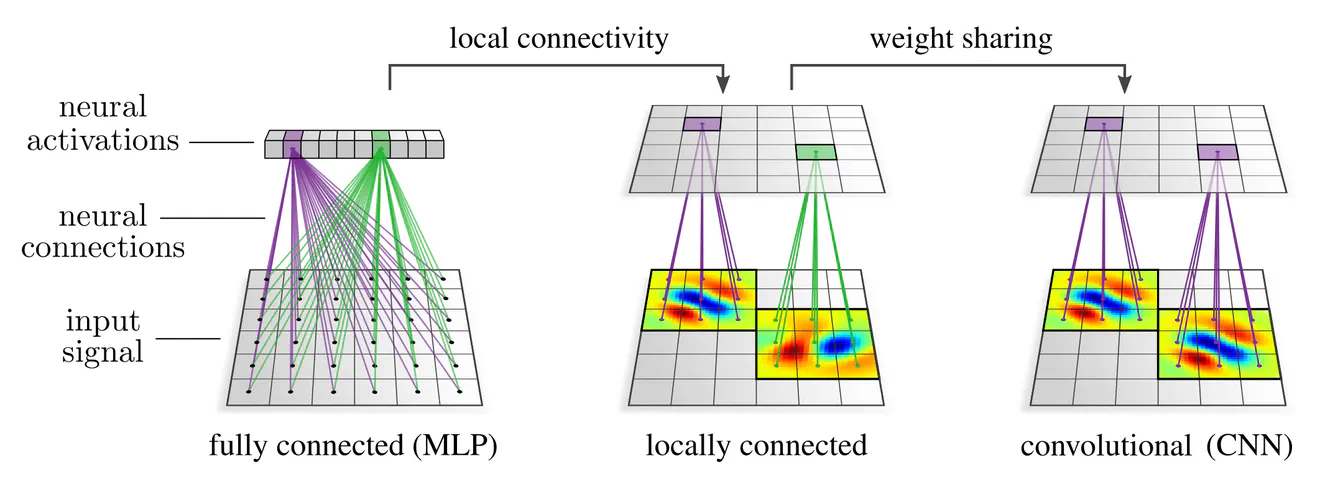
1. Local Connectivity: Instead of connecting every input neuron to every output neuron, neurons in a CNN layer are only connected to a small, localized region of the input. This input region is called the neuron's receptive field. This design preserves the spatial relationships in the data because the network processes the image in local patches.

2. Parameter Sharing (or Weight Sharing): This is the central innovation of CNNs. Instead of learning a separate set of weights for every neuron, we define a single set of weights, called a filter (or kernel), which is shared among all neurons in a given output map. This filter slides across the entire input image, applying the same transformation at every location. This drastically reduces the number of parameters and makes the computation location-independent.

The image below provides an excellent visual comparison of a fully connected network, a locally connected network (which has local connectivity but no parameter sharing), and a convolutional network.

The Convolution Operation

The mechanism that implements local connectivity and parameter sharing is the convolution operation. In a CNN, a convolution involves sliding a small filter over the input image and, at each location, computing the dot product between the filter's weights and the corresponding pixels in the image patch.

Let's formalize this. For a 2D input image $I$ and a 2D kernel $K$, the discrete convolution operation at a location $(i,j)$ is defined as:

$$(I\ast K)[i,j]=\sum _m\sum _{n}I[i-m,j-n]K[m,n]$$

This operation produces a 2D output called a feature map or an activation map. Each element in the feature map corresponds to the response of that filter at a particular location in the input. A high activation means the feature that the filter is looking for (e.g., a vertical edge) is present at that location.

The following video provides an intuitive and mathematical walkthrough of this process.

In practice, a convolutional layer applies not just one, but multiple filters to the input. Each filter learns to detect a different feature. If we use 64 different filters, we will produce 64 corresponding feature maps. These maps are stacked together to form the output volume, which then serves as the input to the next layer.

Learning Spatial Hierarchies

The true power of CNNs emerges when we stack these convolutional layers. Each layer learns to detect features of increasing complexity, forming a spatial hierarchy.

• Layer 1: The first layer operates directly on the raw pixels. Its filters learn to detect very simple patterns, such as oriented edges, color gradients, and simple textures.
• Layer 2: This layer takes the feature maps from the first layer as its input. Its filters learn to combine the simple patterns into more complex motifs, like corners (combining a horizontal and a vertical edge), textures, or simple curves.
• Deeper Layers: Subsequent layers continue this process, combining features from previous layers into ever more abstract and complex concepts. They might learn to detect object parts like eyes, noses, or wheels, and eventually, higher layers can respond to entire objects like faces or cars.

This hierarchical decomposition of the visual world is a remarkably effective strategy for object recognition. The following video provides a compelling visualization of the features learned at different layers of a CNN trained for face detection.

The Theoretical Motivation: Translation Equivariance

We've seen that parameter sharing makes CNNs efficient. However, its most profound consequence is a property called translation equivariance.

An operation is equivariant to translation if shifting the input results in an equivalent shift in the output. For a convolutional layer $\mathcal{L}$ and a translation operation $T$, this means:

$$\mathcal{L}(T(I))=T(\mathcal{L}(I))$$

In simpler terms, if a cat is in the top-left of an image, the "cat detector" features will activate in the top-left of the feature map. If we move the cat to the bottom-right, the same "cat detector" features will activate in the bottom-right of the feature map.

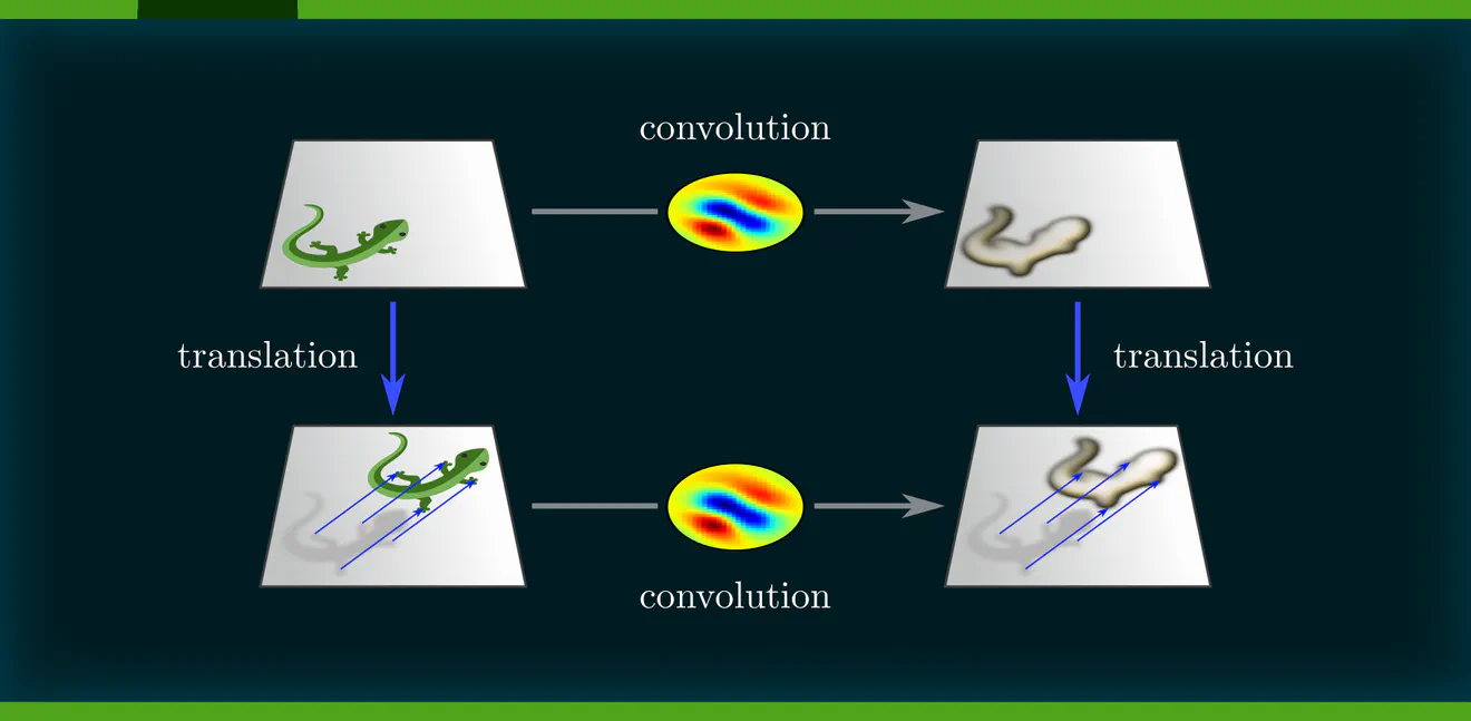
This property is a direct result of parameter sharing. Because the same filter is applied everywhere, the network's ability to detect a feature is independent of its location. This is an incredibly powerful inductive bias for vision tasks, as an object's identity does not change when it moves across the frame.

The relationship between parameter sharing and equivariance is, in fact, fundamental. You can see it as two sides of the same coin. While we often think of parameter sharing as a design choice that implies equivariance, we can also take a more theoretical stance: if we demand that our neural network layer be translation equivariant, we can mathematically prove that its linear operations must be convolutions (i.e., they must share parameters).

This deeper connection is explored beautifully in the following article.

Conclusion

In this lesson, we have moved from general-purpose feedforward networks to a specialized architecture designed for spatial data. We have seen how CNNs overcome the limitations of MLPs for image processing through the principles of local connectivity and parameter sharing.

Here are the key takeaways:

• Convolutional Neural Networks (CNNs) are designed to process data with a grid-like topology, such as images.
• They use local connectivity, where neurons only respond to a small local region of the input, preserving spatial structure.
• The core mechanism is the convolution operation, where a learnable filter (kernel) slides across the input to produce a feature map.
• Parameter sharing—using the same filter at all locations—drastically reduces the parameter count and, more importantly, endows the network with translation equivariance.
• This equivariance means the network can detect features regardless of their position, a powerful assumption for visual tasks.
• By stacking convolutional layers, CNNs learn a hierarchy of features, progressing from simple edges and textures to complex object parts and entire objects.

In our next lesson, we will complete our picture of the standard CNN architecture by examining the roles of pooling layers, stride, and padding. These components are used to control the spatial dimensions of the feature maps and build larger receptive fields, further enhancing the network's ability to learn from spatial hierarchies.