LSTMs & GRUs: Conquering Vanishing Gradients with Gates

Introduction

In our previous lesson, we undertook a deep dive into the mechanics of training vanilla Recurrent Neural Networks. We derived Backpropagation Through Time (BPTT) and uncovered the mathematical origins of the vanishing and exploding gradient problems. The core issue, as we established, is the repeated multiplication of the recurrent weight matrix $W_{hh}$, which causes the gradient signal to either shrink or grow exponentially over long sequences. This fundamentally limits the ability of vanilla RNNs to learn long-range dependencies.

This lesson introduces the canonical solution to this problem: the Long Short-Term Memory (LSTM) network. We will deconstruct the LSTM architecture to understand its core innovation—the cell state—and the system of "gates" that regulate it. Our primary goal is to describe precisely how this gating mechanism creates an alternative pathway for gradient flow, one that is primarily additive rather than multiplicative. This allows LSTMs to preserve information and transmit gradients over much longer time horizons. We will also examine a popular, streamlined variant, the Gated Recurrent Unit (GRU), and compare its design and trade-offs with the LSTM.

The Core Idea: An Information Superhighway

The fundamental flaw in a vanilla RNN is that the hidden state $h_t$ is forced to serve two masters: it must carry the memory of the entire sequence history, and it must also provide a useful representation for the output at the current time step. The LSTM's crucial insight, first proposed by Hochreiter and Schmidhuber in 1997, is to decouple these roles.

An LSTM unit introduces a new component, the cell state ($C_t$), which acts as a dedicated memory channel or an "information superhighway." This channel runs parallel to the main flow of computation, carrying information across many time steps. Crucially, the LSTM is designed to make only minor, controlled modifications to this cell state, primarily through addition and element-wise multiplication. This structure is the key to preserving the gradient signal.

Let's begin with an intuitive overview of the LSTM architecture and its components. The following video provides an excellent, high-level explanation.

Deconstructing the LSTM Cell

As the video explains, an LSTM unit maintains both a cell state $C_t$ (long-term memory) and a hidden state $h_t$ (short-term memory). The flow of information is controlled by a series of gates. These "gates" are simply neural network layers (typically a linear transformation followed by a sigmoid activation) that learn to regulate what information is forgotten, what is added, and what is outputted.

Let's examine the structure of an LSTM cell, using the diagram below.

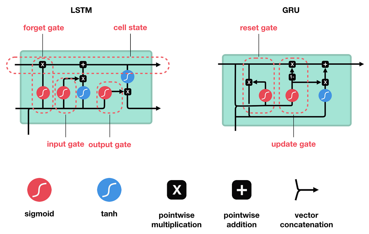
An LSTM cell at time step $t$ takes three inputs: the current input vector $x_t$, the previous hidden state $h_{t-1}$, and the previous cell state $C_{t-1}$. It then produces two outputs: the new hidden state $h_t$ and the new cell state $C_t$. This is accomplished through four interacting components:

1. Forget Gate ($f_t$): This gate decides what information to discard from the previous cell state, $C_{t-1}$. It looks at $h_{t-1}$ and $x_t$ and outputs a number between 0 and 1 for each element in the cell state vector. A 1 represents "completely keep this," while a 0 represents "completely get rid of this."

   $$f_t=\sigma (W_f[h_{t-1},x_t]+b_f)$$

2. Input Gate ($i_t$) and Candidate Cell State (${\tilde{C}}_t$): This two-part mechanism decides what new information to store.

   • First, a tanh layer creates a vector of new candidate values, ${\tilde{C}}_t$, that could be added to the state.
   • Second, the input gate (a sigmoid layer) decides which of these candidate values to update, scaling them by a value between 0 and 1.
   $$i_t=\sigma (W_i[h_{t-1},x_t]+b_i)$$ $${\tilde{C}}_t=\tanh (W_C[h_{t-1},x_t]+b_C)$$

3. Cell State Update: This is the most critical step. The new cell state $C_t$ is calculated by first forgetting some old information and then adding some new information.

   $$C_t=f_t\odot C_{t-1}+i_t\odot {\tilde{C}}_t$$

   Here, $\odot$ denotes element-wise multiplication. Notice the structure: the old state $C_{t-1}$ is multiplied by the forget gate, and the new candidate state ${\tilde{C}}_t$ is multiplied by the input gate. The results are then added together. This additive interaction is the core of the LSTM's solution to the vanishing gradient problem.

4. Output Gate ($o_t$): Finally, this gate determines the new hidden state $h_t$. It takes the updated cell state $C_t$, passes it through a tanh function to squash the values, and then uses a sigmoid gate ($o_t$) to filter which parts of the cell state are exposed as the final hidden state.

   $$o_t=\sigma (W_o[h_{t-1},x_t]+b_o)$$ $$h_t=o_t\odot \tanh (C_t)$$

To solidify your understanding of this mechanism, let's walk through the process with a more detailed, equation-focused video.

The Gradient Highway: Additive vs. Multiplicative Updates

Now we arrive at the central question: how does this architecture solve the vanishing gradient problem? The answer lies in the derivative of the cell state update rule.

Recall from the previous lesson that the gradient backpropagating through a vanilla RNN involved a product of Jacobian matrices:

This repeated multiplication by $W_{hh}$ was the source of the instability.

Now, let's look at the gradient flow through the LSTM's cell state. The update rule is $C_t=f_t\odot C_{t-1}+i_t\odot {\tilde{C}}_t$. When we compute the partial derivative of $C_t$ with respect to $C_{t-1}$ during backpropagation, the chain rule gives us:

This is a remarkably simple result. The gradient flowing from $C_t$ back to $C_{t-1}$ is just element-wise multiplied by the output of the forget gate, $f_t$. There is no multiplication by a shared weight matrix like $W_{hh}$.

When we unroll this over many time steps, the gradient of the loss at time $T$ with respect to the cell state at time $k$ flows through this "highway":

The gradient is propagated by a sequence of element-wise multiplications with the outputs of the forget gates at each step. Because these gates are controlled by sigmoid functions, their values are between 0 and 1. The network can learn to set $f_j\approx 1$ for specific dimensions of the cell state, effectively creating an uninterrupted path for the gradient to flow backward. It can "choose" to remember information by keeping the forget gate open. This prevents the exponential decay that plagued vanilla RNNs.

The following resource provides a rigorous written explanation of this mechanism, including a full derivation of the backpropagation equations for an LSTM cell.

It is important to note that while LSTMs drastically mitigate the vanishing gradient problem, they do not completely eliminate it. If the network learns to set the forget gate to values consistently less than 1 over a very long sequence, the gradient can still diminish. However, the ability to dynamically control this flow at each time step is a monumental improvement.

A Simpler Alternative: The Gated Recurrent Unit (GRU)

In 2014, Cho et al. introduced the Gated Recurrent Unit (GRU) as a simpler alternative to the LSTM. The GRU achieves a similar outcome with a more streamlined architecture, as shown in the right-hand portion of the "LSTM and GRU Architectures" diagram.

The key simplifications are:

1. Combined State: The GRU merges the cell state and hidden state into a single hidden state, $h_t$.
2. Fewer Gates: It uses only two gates instead of three:
   • Update Gate ($z_t$): This gate acts like a combination of the LSTM's forget and input gates. It decides how much of the past information to keep and how much new information to add.
   • Reset Gate ($r_t$): This gate determines how much of the past information to "forget" when computing the candidate new state.

The update equation for a GRU is:

Here, ${\tilde{h}}_t$ is the candidate hidden state. This equation represents a direct interpolation between the previous state $h_{t-1}$ and the candidate state ${\tilde{h}}_t$, controlled by the update gate $z_t$. Like the LSTM, this additive structure allows gradients to flow more easily. If the update gate $z_t$ learns to output values close to 0, the previous hidden state $h_{t-1}$ is passed through almost unchanged, preserving information and its gradient.

In practice, there is no definitive winner between LSTMs and GRUs. LSTMs are more expressive due to their separate cell state, but GRUs are simpler, faster to compute, and have fewer parameters, which can make them easier to train on smaller datasets.

Conclusion

In this lesson, we have dissected the internal workings of LSTMs and GRUs to understand how they address the fundamental limitations of vanilla RNNs.

Key takeaways from this lesson include:

• LSTMs introduce a separate cell state ($C_t$) that acts as an information highway, decoupled from the short-term hidden state ($h_t$).
• The core of the solution is the additive cell state update ($C_t=f_t\odot C_{t-1}+i_t\odot {\tilde{C}}_t$), which allows gradients to flow through time without the exponential decay caused by repeated matrix multiplication.
• Gating mechanisms (forget, input, and output gates) are learnable sub-networks that intelligently control what information is stored, forgotten, and read from the cell state.
• The gradient of the cell state with respect to its previous value is simply the forget gate ($\frac{\partial C_t}{\partial C_{t-1}}=f_t$), allowing the network to learn to preserve gradients by keeping the gate open.
• GRUs are a simplified alternative, combining the cell and hidden states and using only two gates (update and reset) to achieve a similar effect with fewer parameters.

These gated architectures revolutionized our ability to model long sequences, enabling breakthroughs in machine translation, speech recognition, and time-series analysis. However, even they have limitations, particularly with extremely long sequences and the difficulty of parallelizing their sequential computation.

In our next lesson, we will combine these powerful recurrent units into a full encoder-decoder architecture for sequence-to-sequence tasks. In doing so, we will identify a new challenge—the "information bottleneck"—which will motivate the need for an even more powerful mechanism: attention.