BPTT and the Vanishing/Exploding Gradient Problem

Recommended resources

The freely available resources this lesson will direct you to.

Introduction

In our last lesson, we deconstructed the vanilla Recurrent Neural Network, exploring its core architecture: a recurrent loop processing sequences step-by-step, with weight matrices shared across time. We visualized this process by "unrolling" the network, revealing a deep computational graph. However, the forward pass is only half the story. To learn, a network must propagate error signals backward from the loss to its parameters.

This lesson delves into the training process for RNNs. Our primary goal is to derive Backpropagation Through Time (BPTT), the algorithm used to calculate gradients in a recurrent setting. As we unpack its mechanics, we will uncover a fundamental weakness inherent in the vanilla RNN architecture: the long-range dependency problem. You will learn, from a mathematical first-principles standpoint, why vanilla RNNs struggle to connect information over long time intervals, leading to the infamous issues of vanishing and exploding gradients.

Deriving Backpropagation Through Time (BPTT)

Backpropagation Through Time is not a new algorithm, but rather the standard backpropagation algorithm applied to the unrolled RNN computational graph. Since the same weight matrices are used at every time step, the gradient of the loss with respect to a given weight is the sum of its gradient contributions from every time step.

Let's define our total loss $L$ for a sequence of length $T$ as the sum of the losses at each time step:

L = t = 1 \sum T L_{t}

Our objective is to find the partial derivatives of $L$ with respect to our parameters: $W_{h y}$ , $b_{y}$ , $W_{x h}$ , $W_{hh}$ , and $b_{h}$ .

Calculating the gradient for the output weights, $\frac{\partial L}{\partial W _{h y}}$ , is straightforward. The loss at time $t$ , $L_{t}$ , depends on $W_{h y}$ only through the output $y_{t}$ , which itself depends on $h_{t}$ . The total gradient is simply the sum of these local contributions:

\frac{\partial L}{\partial W _{h y}} = t = 1 \sum T \frac{\partial L _{t}}{\partial W _{h y}}

The calculation for the recurrent and input weights ( $W_{hh}$ and $W_{x h}$ ) is more involved. A change to $W_{hh}$ at time step $k$ affects the hidden state $h_{k}$ , which in turn influences all subsequent hidden states $h_{k + 1}, h_{k + 2}, \dots, h_{T}$ and their corresponding losses. Therefore, to calculate the full gradient $\frac{\partial L}{\partial W _{hh}}$ , we must sum up these influences across all time.

The following resource provides a detailed, step-by-step derivation. Given your background in multivariable calculus, the application of the chain rule should be familiar.

Backpropagation Through Time for Recurrent Neural Network

This article provides a rigorous mathematical derivation of BPTT. It systematically calculates the gradients for each parameter matrix.

Read from the beginning, starting with the BPTT introduction, down to the start of the "Vanishing/Exploding Gradients" section. Pay close attention to the derivations for the recurrent weights (W_{hh}) and the input weights (W_{xh}). The most critical insight is how the chain rule is applied recursively to calculate the influence of a past hidden state h_k on a future one h_t. Notice the emergence of this product term: \frac{\partial h_{t+1}}{\partial h_k} = \prod_{j=k}^{t} \frac{\partial h_{j+1}}{\partial h_j} This product of Jacobian matrices is the key to understanding the challenges of training RNNs.

The Gradient Product Problem: Vanishing and Exploding

The BPTT derivation reveals that the gradient signal from a loss at time $t$ must travel backward through a chain of matrix multiplications to update weights at an earlier time $k$ . This "path" is governed by the product of Jacobians we just identified. Let's analyze the term inside the product:

\frac{\partial h _{j + 1}}{\partial h _{j}} = \frac{\partial tanh ( W _{x h} x _{j + 1} + W _{hh} h _{j} + b _{h} )}{\partial h _{j}}

Using the chain rule, this becomes:

\frac{\partial h _{j + 1}}{\partial h _{j}} = diag (tanh^{'} (z_{j + 1})) W_{hh}

where $z_{j + 1}$ is the pre-activation input to the $tanh$ function at step $j + 1$ , and $tanh^{'}$ is its derivative.

The gradient flowing from step $t$ back to $k$ is therefore proportional to a product of $t - k$ such matrices. This multiplicative structure is the source of a profound instability.

A conceptual sketch of how the magnitude of the gradient (derivative size) changes as it propagates backward in time. In the exploding case, it grows uncontrollably. In the vanishing case, it shrinks to zero.

Mathematical Origins of the Problem

The behavior of this long product of matrices is determined by two key factors: the recurrent weight matrix $W_{hh}$ and the derivative of the activation function.

Saturating Activation Function: The derivative of the hyperbolic tangent, $tanh^{'} (z) = 1 - tanh^{2} (z)$ , has a maximum value of 1 (at $z = 0$ ) and approaches 0 as $∣ z ∣$ gets large. This is known as a saturating nonlinearity. In practice, the hidden state activations are often not close to zero, so this derivative term is almost always a value strictly less than 1. Each step of the backpropagation journey multiplies the gradient by a factor less than one, pushing it exponentially towards zero.
Repeated Multiplication of $W_{hh}$ : The core of the problem lies in the repeated multiplication by the same matrix, $W_{hh}$ . From linear algebra, we know that the long-term behavior of repeatedly multiplying a vector by a matrix is governed by the matrix's eigenvalues. If $W_{hh}$ is diagonalizable, any vector can be expressed in the basis of its eigenvectors. After $n$ multiplications, the component of the vector along each eigenvector $v_{i}$ will be scaled by $λ_{i}^{n}$ , where $λ_{i}$ is the corresponding eigenvalue.
- If the largest eigenvalue in magnitude (the spectral radius, $ρ (W_{hh})$ ) is greater than 1, gradients will tend to grow exponentially as they are propagated backward. This is the exploding gradient problem.
- If the spectral radius is less than 1, gradients will tend to shrink exponentially. This is the vanishing gradient problem.

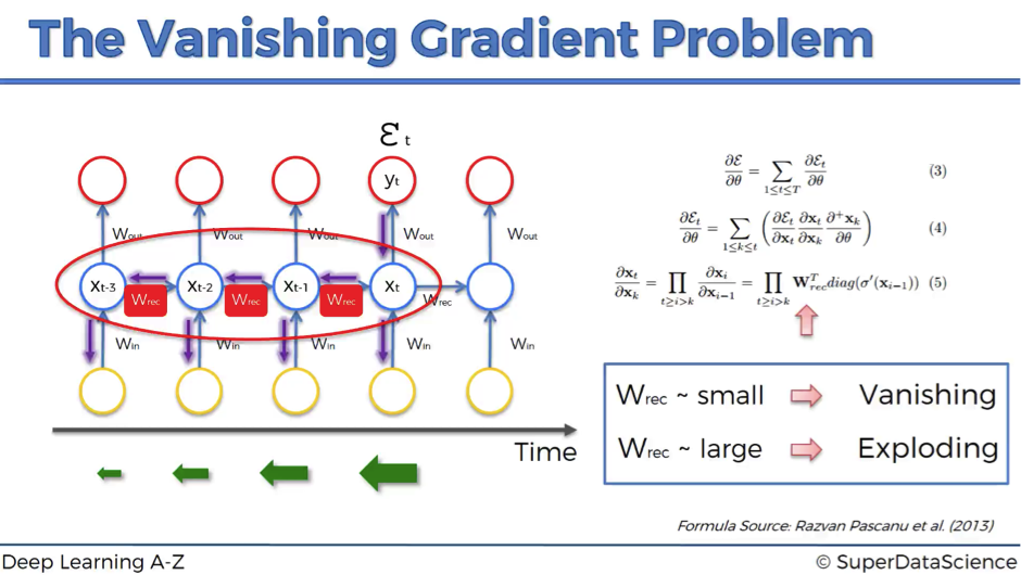
This diagram illustrates the core mechanism. The gradient signal must propagate backward through time, repeatedly being multiplied by the recurrent weights $W_{rec}$ (our $W_{hh}$). The size of these weights determines whether the signal vanishes or explodes.

Combining these two effects, the gradient vanishes almost by default. The $tanh^{'}$ term systematically shrinks the gradient, so unless the spectral radius of $W_{hh}$ is carefully balanced to be greater than 1 to counteract this shrinkage, the gradient signal will decay to zero over long distances. In practice, maintaining this balance is extremely difficult, making vanishing gradients the more pervasive and challenging issue.

The following video provides an excellent and mathematically rigorous explanation of this phenomenon, leveraging concepts from linear algebra that should be familiar to you.

Vanishing Gradients: Why Training RNNs is Hard

This video, "Vanishing Gradients: Why Training RNNs is Hard," walks through the BPTT derivation and then provides a deep analysis of the conditions for vanishing and exploding gradients.

First, watch from this segment to see the derivation of the gradient contribution, highlighting the repeated multiplication of the Jacobian term (which the presenter calls \Omega). Then, continue with the more rigorous analysis from this point. This section masterfully connects the problem to the eigenvalues and spectral radius of the weight matrix, using concepts like diagonalization and change of basis to explain the exponential scaling.

The Long-Range Dependency and Credit Assignment Problems

The mathematical consequence of vanishing gradients is a practical inability to learn long-range dependencies. Imagine a language modeling task where a verb at the end of a long sentence must agree with a subject at the beginning.

"The cat, which for many years lived in the old house at the end of the lane and was known by all the neighbors for its peculiar habits, was finally adopted."

To correctly predict "was" instead of "were", the model needs to connect it to the singular subject "cat" from many words ago. During training, the error signal from the prediction "was" must propagate back through every intermediate word to reach "cat". Because of vanishing gradients, this signal will have decayed to effectively zero long before it reaches the early parts of thesentence. The weight updates that would strengthen the "cat -> was" connection never occur.

This is a specific instance of the broader credit assignment problem: how do we assign responsibility (credit or blame) for an output to the numerous decisions (parameter settings) that produced it? For vanilla RNNs, the vanishing gradient means credit can only be assigned to recent events. The network becomes myopic, capable of learning local patterns but blind to long-term context.

The following resource provides an exceptional, in-depth discussion of this problem, including empirical evidence from classic tasks where vanilla RNNs fail.

Vanishing Gradients in RNNs: Why Neural Networks Forget Long ...

This article explores the vanishing gradient problem from multiple angles: theoretical, mathematical, and empirical.

Please read the following sections: Start with The Gradient Product Problem for a clear framing of the issue. Continue to Eigenvalue Analysis, which provides a deeper mathematical perspective on why the products shrink or explode. Read the section on how saturating activations contribute to the problem. Then, read about the consequences, which formalizes the "memory horizon" of an RNN. Finally, review the empirical evidence and the intuitive explanation of the credit assignment problem. This will ground the theory in concrete examples.

While exploding gradients are also a problem, they are often easier to deal with. Because they result in huge, unstable weight updates and NaN (Not a Number) values in the loss, they are easy to detect. A common and effective heuristic is gradient clipping, where the norm of the gradient is simply capped at a certain threshold before the weight update. If $∥ g ∥ > θ$ , then $g \leftarrow \frac{θ}{∥ g ∥} g$ . This doesn't solve the underlying instability, but it prevents the optimization process from diverging. Vanishing gradients, by contrast, are silent; the model simply fails to learn, with no obvious error message.

Conclusion

In this lesson, we have moved from the architecture of RNNs to the mechanics of their training, and in doing so, uncovered a critical flaw.

Key takeaways from this lesson include:

Backpropagation Through Time (BPTT) is the application of the chain rule to the unrolled RNN graph. Gradients for shared weights are summed across all time steps.
The BPTT derivation reveals that gradient information from the past is transmitted via a product of Jacobian matrices.
This multiplicative structure leads to exploding and vanishing gradients. The problem is rooted in the repeated multiplication of the recurrent weight matrix $W_{hh}$ and the derivatives of the activation function, which are often $\leq 1$ .
Vanishing gradients make it practically impossible for vanilla RNNs to learn long-range dependencies, as the "credit" for an output cannot be assigned to events that occurred far in the past.

The limitations of the vanilla RNN are not just a minor inconvenience; they fundamentally restrict its modeling power. The multiplicative nature of the recurrence relation is both its strength (allowing it to process sequences) and its weakness (causing gradient instability). This realization spurred the development of new architectures designed explicitly to overcome this problem.

In our next lesson, we will investigate the most successful of these solutions: the Long Short-Term Memory (LSTM) network. You will see how its introduction of a "cell state" and explicit "gating mechanisms" creates an alternative path for information, relying on additive interactions that allow gradients to flow much more freely through time.