Mesh Analysis: KVL Equations

Hello! Let's continue our journey into Mesh Analysis.

In our last lesson, we established the "setup" phase of this powerful technique. We learned how to identify meshes as the "window panes" of a planar circuit and how to assign a conceptual mesh current to each one. Crucially, we saw that the physical current in any branch is simply the superposition of the mesh currents flowing through it.

Today, we move to the heart of the method. We will combine our mesh current variables with Kirchhoff's Voltage Law (KVL) to build a system of equations. Your goal for this lesson is to learn how to formulate KVL equations for each mesh by expressing voltage changes in terms of mesh currents. By the end, you'll be able to take any resistive circuit, no matter how complex, and translate it into a set of solvable algebraic equations.

A Quick Refresher: The "Why" of KVL

Before we get into the mechanics, let's anchor ourselves in the physical principle. As you appreciate understanding the "why" behind the rules, it's worth remembering what KVL truly represents.

In short, KVL states that the sum of all voltage drops and rises around any closed loop must equal zero. This is because voltage is potential energy per charge. If you move a charge around a loop and return to the starting point, its net change in potential energy must be zero. Any energy it gained from sources must have been perfectly balanced by the energy it lost (dissipated) in components like resistors.

The KVL Recipe for a Mesh

Now, let's build the step-by-step procedure for writing a KVL equation for a single mesh. We will "walk" around the mesh in the same direction as its assigned mesh current (conventionally clockwise).

As we cross each component, we add its voltage change to our equation. To keep things systematic, we will use a consistent sign convention:

• A voltage drop (going from + to -) is a positive term.
• A voltage rise (going from - to +) is a negative term.

The sum of all these terms around the loop must equal zero.

$$\sum V_{\text{drops}}-\sum V_{\text{rises}}=0$$

Let's break this down:

1. Voltage Sources: If we cross a voltage source from the negative to the positive terminal, it's a voltage rise, so we add a negative term (-V). If we cross from positive to negative, it's a drop, so we add a positive term (+V).
2. Resistors in the "Home" Mesh: When we cross a resistor that is only part of the mesh we are analyzing (our "home" mesh), the voltage drop is given by Ohm's Law. Since our path follows the current, it's always a drop. We add a positive term: +IR.
3. Resistors Shared Between Meshes: This is the most critical step. A resistor shared between your "home" mesh (say, with current $I_1$) and an adjacent mesh (with current $I_2$) has a net current flowing through it.
   • The net current in the direction of our travel is ($I_1-I_2$).
   • The voltage drop across this resistor is therefore R * (I_1 - I_2). We add this as a positive term to our KVL equation for mesh 1.

The following video provides an exceptionally clear, step-by-step demonstration of writing the KVL equation for the first mesh in a circuit.

This image provides a static view of the key idea for shared components.

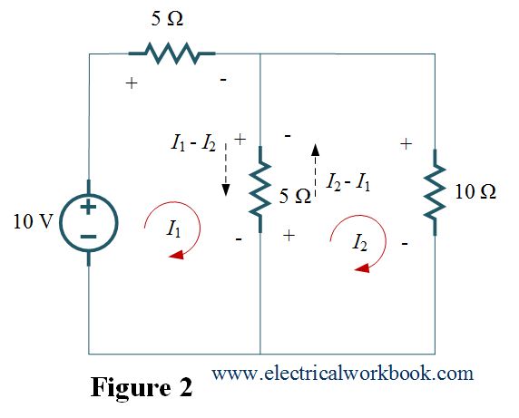
Applying the Recipe to Adjacent Meshes

Once we have the KVL equation for the first mesh, we simply repeat the process for every other mesh in the circuit. Let's consider writing the equation for the adjacent mesh, Mesh B, from the video.

We now walk clockwise around Mesh B, following the path of current $I_B$.

• For resistors only in Mesh B (like the 6Ω resistor), the voltage drop is straightforward: +6 * I_B.
• Now we come to the 8Ω resistor shared with Mesh A. This time, our direction of travel is up through the resistor, following $I_B$. The opposing current is $I_A$, which flows down.
• The net current in our direction of travel (upwards) is now ($I_B-I_A$).
• The voltage drop term for our Mesh B equation is +8 * (I_B - I_A).

Notice the symmetry: In the Mesh A equation, the term was R * (I_A - I_B). In the Mesh B equation, it becomes R * (I_B - I_A). The "home" current is always first (and positive) in the subtraction.

Let's see this applied in a different example.

From Equations to a System

By repeating this process for every mesh, you generate one KVL equation per mesh. If you have M meshes, you will have M linear equations with M unknown mesh currents ($I_1,I_2,...,I_M$).

For a two-mesh circuit, your final, simplified equations will look something like this:
$a{I}_1+b{I}_2=V_a$
$c{I}_1+d{I}_2=V_b$

This is a system of linear equations. Given your algebra background, you know this can be solved systematically. A common and efficient way, especially for more than two meshes, is to use matrices.

While we will focus on solving these systems later, recognizing this structure is important. It confirms that mesh analysis provides a direct, systematic path from a circuit diagram to a solvable mathematical problem.

Conclusion

You have now learned the complete procedure for formulating the equations of mesh analysis. This is the most crucial part of the method; the rest is algebra.

Key Takeaways:

• Mesh analysis uses KVL to generate one independent equation for each mesh in a circuit.
• To write an equation, "walk" around the mesh and sum the voltage changes, setting the total to zero. A voltage drop is treated as positive, and a voltage rise as negative.
• The voltage drop across a shared resistor R between a "home" mesh H and an "adjacent" mesh A is given by R * (I_H - I_A).
• This process results in a system of M linear equations for M unknown mesh currents, which can be systematically solved.

Preview of the Next Lesson:
We've built a robust method for circuits with resistors and voltage sources. But what happens if there's a current source in the circuit? If it's on the edge of a mesh, it's simple. But if it's shared between two meshes, it creates a problem for our KVL walk. In the next lesson, we will introduce the supermesh technique—a powerful extension that is the direct dual of the supernode method you already know—to handle this exact situation.