Matrix Operations and Dimension Verification with NumPy

Hello! Last lesson, you used indexing, broadcasting, and vectorized arithmetic to transform arrays. This lesson keeps the same attention to shape, but changes the operation: matrix multiplication combines rows with columns, rather than multiplying entries in matching positions.

You’ll use NumPy to add, scale, transpose, and multiply matrices, then check dimensions before trusting a result. These checks are useful in machine-learning code, where a feature matrix and a set of weights must fit together. Allow about 40 minutes to read, watch, and run the examples.

Read a shape before doing the calculation

A two-dimensional array has a row axis and a column axis. If its shape is (4, 2), it has four rows, two columns, and eight entries. NumPy reports these properties through .shape, .ndim, and .size.

This picture shows why specifying a new shape requires the same total number of entries:

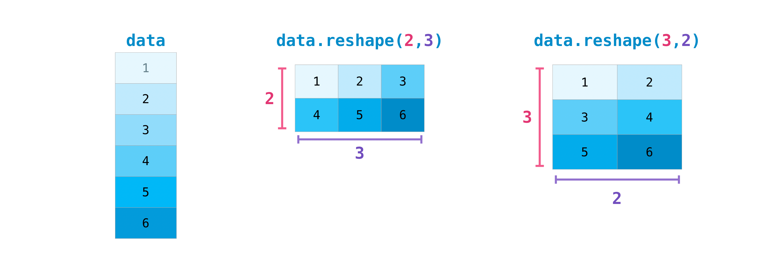
Try both arrangements and a transpose:

import numpy as np

data = np.arange(1, 7)
grid = data.reshape(2, 3)

print(data.shape)             # (6,)
print(grid.shape)             # (2, 3)
print(grid.ndim, grid.size)   # 2 6

print(grid.T)
# [[1 4]
#  [2 5]
#  [3 6]]

print(data.reshape(3, 2))
# [[1 2]
#  [3 4]
#  [5 6]]

Both outputs at the end have shape (3, 2), but they contain different arrangements. Transpose exchanges rows and columns; reshape assigns a new shape while traversing the entries in their existing order by default. Equal output shapes do not guarantee equal output values.

Distinguish entry-wise arithmetic from matrix multiplication

Addition and subtraction operate on corresponding entries of equally shaped matrices. Multiplication by a single number scales every entry. NumPy’s * also multiplies entry by entry—it does not perform a matrix product.

Here is a version you can run and inspect:

A = np.array([[1, 2],
              [3, 4]])
B = np.array([[5, 6],
              [7, 8]])

print(A + B)       # [[ 6  8]
                   #  [10 12]]
print(2 * A)       # [[2 4]
                   #  [6 8]]
print(A * B)       # [[ 5 12]
                   #  [21 32]]
print(A @ B)       # [[19 22]
                   #  [43 50]]

The top-left entry of A * B is 1 * 5, or 5. The top-left entry of A @ B is the sum of products from A’s first row and B’s first column: $1(5)+2(7)=19$. Thus, choosing * instead of @ can produce a plausible-looking array with the wrong meaning.

For matrix addition in a numerical program, checking for identical shapes is a sensible precaution. NumPy also permits some differently shaped arrays to combine through broadcasting, as you saw last lesson; that behavior may not represent the pairwise matrix addition you intended.

Predict a matrix product’s dimensions

For two-dimensional matrices, the number of columns in the left matrix must equal the number of rows in the right matrix. If left.shape is (n, k) and right.shape is (k, m), their product has shape (n, m). Each output entry combines one length-k row with one length-k column.

Watch a short calculation in Python NumPy | Dot Product by Automation Helpers:

Now apply the rule to a small feature calculation. Reuse the four-observation, two-feature array from last lesson. Let each column of W contain weights for one output:

X = np.array([[2., 4.],
              [4., 6.],
              [6., 8.],
              [8., 10.]])       # (4, 2): observations, features

W = np.array([[ 1., -1., 0.],
              [0.5,  2., 1.]])  # (2, 3): features, outputs

scores = X @ W
print(scores.shape)             # (4, 3)
print(scores[0])                # [4. 6. 4.]

The shared dimension is 2: each output combines two features. The first observation [2., 4.] produces 4. in the first output column because $2(1)+4(0.5)=4$. Its second output is $2(-1)+4(2)=6$. Four observations remain four rows; three weight columns produce three output columns.

Order matters. X @ W is valid, but W @ X is not: the left operand would have three columns while the right has four rows. Even when both orders are valid, they generally yield different values.

Handle vectors without losing track of axes

In NumPy, a one-dimensional vector of length two has shape (2,). It is not, by itself, a two-dimensional row matrix (1, 2) or column matrix (2, 1). Consequently, .T does not change a one-dimensional vector’s shape.

weights = np.array([1., 0.5])

predictions = X @ weights
print(weights.shape)       # (2,)
print(weights.T.shape)     # (2,)
print(predictions.shape)   # (4,)
print(predictions)         # [ 4.  7. 10. 13.]

column_weights = weights.reshape(2, 1)
column_predictions = X @ column_weights
print(column_weights.shape)      # (2, 1)
print(column_predictions.shape)  # (4, 1)

These products use the same two weights and give the same numerical prediction for each observation, but their output shapes differ. That distinction matters when later code expects either a flat prediction array or a column of values. If you need a two-dimensional column, construct one explicitly rather than relying on .T to change a one-dimensional array.

Verify before and after multiplying

A useful engineering habit is to check the input contract before @, then check the output contract afterward. This small function is deliberately limited to two-dimensional matrices so its rule is easy to inspect:

def matmul_checked(left, right):
    left = np.asarray(left)
    right = np.asarray(right)

    if left.ndim != 2 or right.ndim != 2:
        raise ValueError("expected two 2-D arrays")
    if left.shape[1] != right.shape[0]:
        raise ValueError(
            f"incompatible shapes: {left.shape} @ {right.shape}"
        )

    result = left @ right
    expected_shape = (left.shape[0], right.shape[1])
    assert result.shape == expected_shape
    return result

checked_scores = matmul_checked(X, W)
np.testing.assert_allclose(checked_scores, scores)

The input checks explain why a multiplication is invalid; the result check records what shape a valid product must have. The final comparison also tests the computed values against the earlier calculation. In a larger numerical project, dimension and value checks help distinguish a mistaken array arrangement from a mistaken calculation.

What to take forward

Use .shape and .ndim to establish what an array represents. Use + and * for entry-wise arithmetic when that is your intent; use @ for a matrix product. Before multiplying two matrices, match the left column count to the right row count and predict the output’s rows and columns. Remember that reshaping, transposing, and using a one-dimensional vector can change—or preserve—axes in different ways.

Next, you’ll load and inspect tabular data with pandas. The same habit of checking dimensions will help you tell observations, features, and missing values apart before modeling.