Recommended resources
The freely available resources this lesson will direct you to.
Welcome back! Over the last two lessons, we've built a highly optimized Union-Find data structure. First, we implemented path compression to flatten our trees during find operations. Then, we added union by rank/size to build balanced, shallow trees during union operations. We've constructed the engine; now it's time to understand its performance specifications.
Today's lesson addresses the learning outcome: Analyze the amortized time complexity of the optimized Union-Find operations. This is the theoretical payoff for the optimizations we've implemented. We will explore what "amortized complexity" means, discover the remarkable speed of our data structure, and frame this knowledge in a way that's practical and powerful for coding interviews.
Worst-Case vs. Amortized Analysis
Let's first consider the worst-case cost of a single find operation. Even with our optimizations, it's possible to have a tree where the height is O(log N). If we call find on a leaf node for the very first time, we might have to traverse O(log N) parent pointers to reach the root. This is the worst-case complexity of a single operation.
However, that expensive operation does something remarkable. Path compression flattens the tree for every node it visits. Subsequent find calls on any of those nodes will now be much faster, potentially O(1). The initial expensive operation has effectively "paid for" the efficiency of future operations.
This is the perfect scenario for amortized analysis. Unlike average-case analysis, which averages performance over random inputs, amortized analysis provides a performance guarantee for a sequence of operations, even in the worst-case scenario. It smooths out the cost, where expensive operations are rare and create "credit" that pays for many cheap operations.
For a deeper introduction to this concept, the following lecture notes provide a clear distinction.
Lecture 1: Amortized Analysis & Union Find
These notes from the University of Waterloo clearly explain why we sometimes need to look beyond simple worst-case analysis per operation.
Read the sections titled Why Amortized Analysis? (pages 3-5) and Types of amortized analyses (pages 6-8) to understand the core idea. You don't need to dive into the "Potential Method" for now; just grasp the difference between worst-case and amortized thinking.
The Power of Two: The Synergy of Optimizations
When we combine union by rank/size with path compression, the result is more powerful than either optimization on its own.
- Union by rank/size acts proactively. It prevents the creation of degenerate, chain-like trees, ensuring the initial height is at most O(log N).
- Path compression acts reactively. It takes any path that is traversed and flattens it, dramatically reducing the cost of future traversals along that same path.

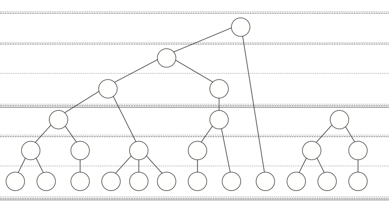
The combination is so effective that the amortized time per operation becomes nearly constant.
The Complexity Result: The Inverse Ackermann Function
The amortized time complexity of the find and union operations in our fully optimized data structure is O(α(N)), where N is the number of elements.
So, what is α(N)? It's the Inverse Ackermann function. While its mathematical definition is complex, its practical implication is incredibly simple: it grows so slowly that for any conceivable input size N you would encounter in computing, α(N) is never greater than 5.
- For N up to , α(N) is 4.
- For N up to , a number far larger than the number of atoms in the universe, α(N) is 5.
Therefore, for all intents and purposes, we can treat O(α(N)) as constant time.
The following video clips provide excellent, concise summaries of this key takeaway, which is exactly how you should think about it in an interview context.
The "Hello Byte" channel gives a very clear and practical summary of the performance of the final, optimized Union-Find.
Watch the final segment from the performance summary. The key message is that the complexity is described by the Inverse Ackermann function, which for all practical purposes makes the operations nearly constant time.
The "take U forward" channel reinforces this same point.
G-46. Disjoint Set | Union by Rank | Union by Size | Path Compression
This clip concisely states the time complexity and explains how to frame it in an interview setting.
Watch the explanation of the final time complexity from the time complexity analysis. It emphasizes that O(4α) is effectively constant.
Building the Intuition (An Easier Bound)
Proving the O(α(N)) bound is famously complex and well beyond the scope of any coding interview. However, we can build some intuition by looking at a slightly simpler, weaker (but still incredibly fast) bound: O(log* N).
The iterated logarithm, written as log* N (pronounced "log star N"), is the number of times you must apply the logarithm function to N before the result is less than or equal to 1.
- log* (2) = 1 (since log₂(2) = 1)
- log* (4) = 2 (since log₂(log₂(4)) = log₂(2) = 1)
- log* (16) = 3 (since log₂(log₂(log₂(16))) = log₂(log₂(4)) = log₂(2) = 1)
- log* (65536) = 4
- log* () = 5
Like α(N), log* N is also practically a constant less than 5 for any real-world value of N. The formal analysis uses a clever "charging" scheme (part of the accounting method of amortized analysis) where nodes are grouped by their rank. The analysis shows that any single node can only "be paid for" a few times before its parent is in a much higher group, after which it's no longer charged. While we won't do the full proof, understanding this intermediate O(log* N) bound helps demystify how these super-slow-growing functions arise in the analysis.
The lecture notes from Waterloo walk through this O(log* N) proof. You are not expected to reproduce this, but skimming it can provide a taste of how such an analysis works.
Lecture 1: Amortized Analysis & Union Find
This section presents a simplified (but still formal) proof for an O(log* N) amortized bound, which is a step toward the full O(α(N)) analysis.
Skim through the section titled Analysis (pages 46-72). Focus on the high-level ideas: The definition of log* N. The idea of grouping elements by their rank (page 58). The charging scheme (page 60), where the cost of a FIND is distributed between the operation itself and the nodes on the path. The goal is not to memorize the math, but to appreciate the technique used to prove that the total cost over many operations is very low.
Summary of Complexities
Let's summarize how our optimizations have improved the data structure.
| Implementation | find Operation |
union Operation |
|---|---|---|
| Naive (long chain) | O(N) | O(1) or O(N) |
| Union by Rank/Size only | O(log N) | O(log N) |
| Union by Rank/Size + Path Compression | O(α(N)) | O(α(N)) |
This table makes it clear why the combination of both optimizations is critical. Together, they deliver the nearly constant time performance that makes Union-Find so powerful.
Conclusion
In this lesson, we analyzed the remarkable efficiency of our fully optimized Union-Find data structure. While a single operation can sometimes be slow, its self-optimizing nature ensures that a sequence of operations is extremely fast.
Key Takeaways:
- Amortized Analysis: Averages the cost of operations over a worst-case sequence, allowing expensive operations to "pay for" future cheap ones.
- O(α(N)) Complexity: The combination of path compression and union by rank/size gives an amortized time complexity of O(α(N)).
- The Inverse Ackermann Function (α(N)): This function grows so slowly that for all practical purposes, it can be considered a small constant (e.g., less than 5).
- The Interview Answer: For a coding interview, it is sufficient to state that the amortized complexity is O(α(N)) and that this is "effectively constant time." Explaining why (the synergy between the two optimizations) demonstrates a deep understanding.
We have now fully developed and analyzed the Union-Find data structure. In the next lesson, we will begin to apply it to solve real problems, starting with its classic use case: applying Union-Find to determine the number of connected components in a graph.