Counting Connected Components with Union-Find

In our last lesson, we explored the impressive performance of our fully optimized Union-Find data structure, culminating in the nearly constant O(α(N)) amortized time complexity for its operations. Now that we have a solid grasp of how this engine works and how efficient it is, we can shift our focus from building the tool to using it.

Today, we'll tackle the first and most classic application of this data structure. This lesson directly addresses the learning outcome: Apply Union-Find to determine the number of connected components in a graph. We will see how the abstract concepts of sets and merging map perfectly to the tangible ideas of nodes and edges, providing an elegant and efficient solution to a fundamental graph problem.

The Problem: Counting Connected Components

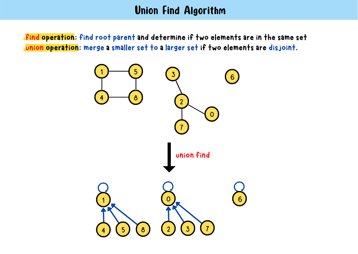
Imagine a social network. Some people are friends with each other, forming groups or "cliques." A person can belong to only one such group. A connected component in a graph is a subgraph in which any two vertices are connected to each other by paths, and which is connected to no additional vertices in the supergraph. Our goal is to count how many of these separate groups exist.

Mapping Graphs to Disjoint Sets

The Union-Find data structure is a natural fit for this problem. The mapping is direct and intuitive:

• Elements in our DSU are the nodes (or vertices) of the graph.
• A disjoint set in our DSU represents a connected component. The root of the set's tree acts as the representative for that entire component.
• An edge (u, v) in the graph is an instruction to perform a union operation on nodes u and v. This merges their respective components.

With this mapping, the algorithm for counting components becomes straightforward:

1. Initialization: Given a graph with N nodes, we initialize a Union-Find data structure with N elements. Initially, each node is in its own set, representing that it is its own component. Therefore, we start with a component_count = N.
2. Process Edges: We iterate through each edge (u, v) in the graph.
3. Union and Count: For each edge, we attempt to union the sets containing u and v. The key insight is this: if find(u) and find(v) return different roots, it means u and v were in different components. The union operation will merge these two components into one. Consequently, the total number of connected components decreases by one. We decrement our component_count.
4. Redundant Edges: If find(u) and find(v) return the same root, the nodes are already in the same component. The edge is redundant and provides no new connectivity information. We do nothing to our component_count.
5. Final Result: After processing all edges, the final value of component_count is the answer.

A Guided Walkthrough

The NeetCode video on this topic provides an excellent step-by-step walkthrough of this exact logic. It solves LeetCode problem 323, "Number of Connected Components in an Undirected Graph," which is precisely our learning goal.

Implementation and Analysis

Now that you've seen the logic, let's examine a complete, clean implementation. The following resource provides a Python solution for a very similar problem, LeetCode 547 "Number of Provinces," which uses an adjacency matrix instead of an edge list but follows the exact same Union-Find principle.

Complexity Analysis

Let's analyze the performance of this approach for a graph with N nodes and E edges.

• Time Complexity:

  • DSU Initialization: O(N) to create and initialize the parent and rank/size arrays.
  • Edge Processing: We loop through E edges. For each edge, we perform one union operation, which internally makes two find calls. The amortized cost of this is O(α(N)). Thus, processing all edges takes O(E * α(N)).
  • Total: The overall time complexity is O(N + E * α(N)). Since α(N) is practically constant, we can consider this to be linear time, O(N + E).

• Space Complexity: O(N) to store the parent and rank/size arrays for the N nodes.

When to Prefer Union-Find over DFS/BFS

As noted in the NeetCode video, you can also solve this problem with a standard graph traversal like Depth-First Search (DFS) or Breadth-First Search (BFS). The time and space complexity for a traversal-based solution is also O(N + E). So, for a static graph given to you all at once, both methods are excellent.

The true power of Union-Find shines in dynamic scenarios. Imagine you are given the nodes, but the edges are arriving one by one in a stream. After each new edge is added, you might be asked: "How many components are there now?" or "Are nodes x and y connected now?"

• A DFS/BFS approach would be inefficient. Each time a new edge arrives, you would have to potentially rebuild your adjacency list and run the entire traversal again, which is O(N+E).
• The Union-Find approach is ideal. Adding an edge is just a single, nearly constant time union operation. You can update the component count in O(α(N)) time. This allows you to answer queries about connectivity and component count in real-time as the graph evolves.

The "take U forward" channel explains this specific use case very well.

Conclusion

In this lesson, we put our Union-Find data structure to work on its most fundamental application: counting connected components in a graph. We saw that by mapping nodes to elements and edges to union operations, we can devise an elegant and highly efficient algorithm.

Key Takeaways:

• Algorithm: Initialize a component count to N. For each edge (u, v), if u and v are not already in the same set, perform a union and decrement the component count.
• Time Complexity: The algorithm runs in O(N + E * α(N)), which is effectively linear time.
• Key Advantage: While comparable to DFS/BFS for static graphs, Union-Find is vastly superior for dynamic graphs where edges are added over time and intermediate connectivity queries are required.

This idea of using find operations to check for existing connectivity before performing a union is a powerful pattern. In our next lesson, we will build directly on this concept to solve a common category of interview problems known as redundant connection problems.