Understanding Union-Find: Core Operations

Recommended resources

The freely available resources this lesson will direct you to.

Welcome to the first lesson in our module on the Union-Find data structure. In the previous module, we concluded our exploration of Tries by analyzing their time and space complexity. We're now shifting to a completely different but equally powerful data structure that excels at managing dynamic groups of elements.

Today, your goal is to explain the Union-Find data structure and its core find and union operations. We will focus on the fundamental concepts: what problem this structure solves, how it's conceptually modeled, and how a basic version of its core operations can be implemented. This foundational understanding is crucial before we explore the optimizations that make this data structure so efficient in later lessons.

What are Disjoint Sets?

Imagine you have a collection of items, and you want to group them into sets where no item belongs to more than one set. These non-overlapping sets are called disjoint sets. The Union-Find data structure, also known as Disjoint Set Union (DSU), is specifically designed to manage such collections.

It is particularly useful for problems involving connectivity and partitioning. For example, given a set of nodes in a graph, we can use Union-Find to keep track of its connected components. Initially, each node is in its own component (its own set). As we add edges, we merge, or "union," the components of the connected nodes.

The data structure primarily supports two critical operations:

Find: Determine which set a particular element belongs to.
Union: Merge two sets into a single new set.

The following video by Abdul Bari provides an excellent introduction to this concept, using a graph-based example to illustrate what Find and Union mean in a practical context.

1.12 Disjoint Sets Data Structure - Weighted Union and Collapsing Find

This video introduces the concept of disjoint sets and their operations.

Watch the segment from the beginning until the explanation of cycle detection. Focus on: How the components of a graph are represented as disjoint sets. The conceptual meaning of the find operation (which set does a vertex belong to?). The condition for performing a union operation (when an edge connects vertices in different sets).

Conceptual Model: A Forest of Trees

The most common way to visualize a collection of disjoint sets is as a forest, which is a collection of trees. Each tree in the forest represents a single disjoint set.

Representative: The root of each tree serves as the unique identifier or representative of that set.
Set Membership: An element belongs to a set if it is a node within that set's corresponding tree.

To perform the core operations within this model:

find(element): To find which set an element belongs to, we traverse up the tree from that element's node until we reach the root. The root is the representative of the set.
union(element1, element2): To merge the sets containing two elements, we first find the representatives (roots) of their respective trees. If the roots are different, we merge the trees by making one root the child of the other.

This image illustrates three disjoint sets, each represented as a tree. The elements {E, L, F}, {I, C, D, K, J, A, B}, and {G, H} form three distinct sets. The roots C, E, and G act as the representatives for their respective sets.

A Naive Implementation: The Parent Array

While the forest model is a great mental picture, the actual implementation is surprisingly simple. We can represent the entire forest using a single array, which we'll call parent.

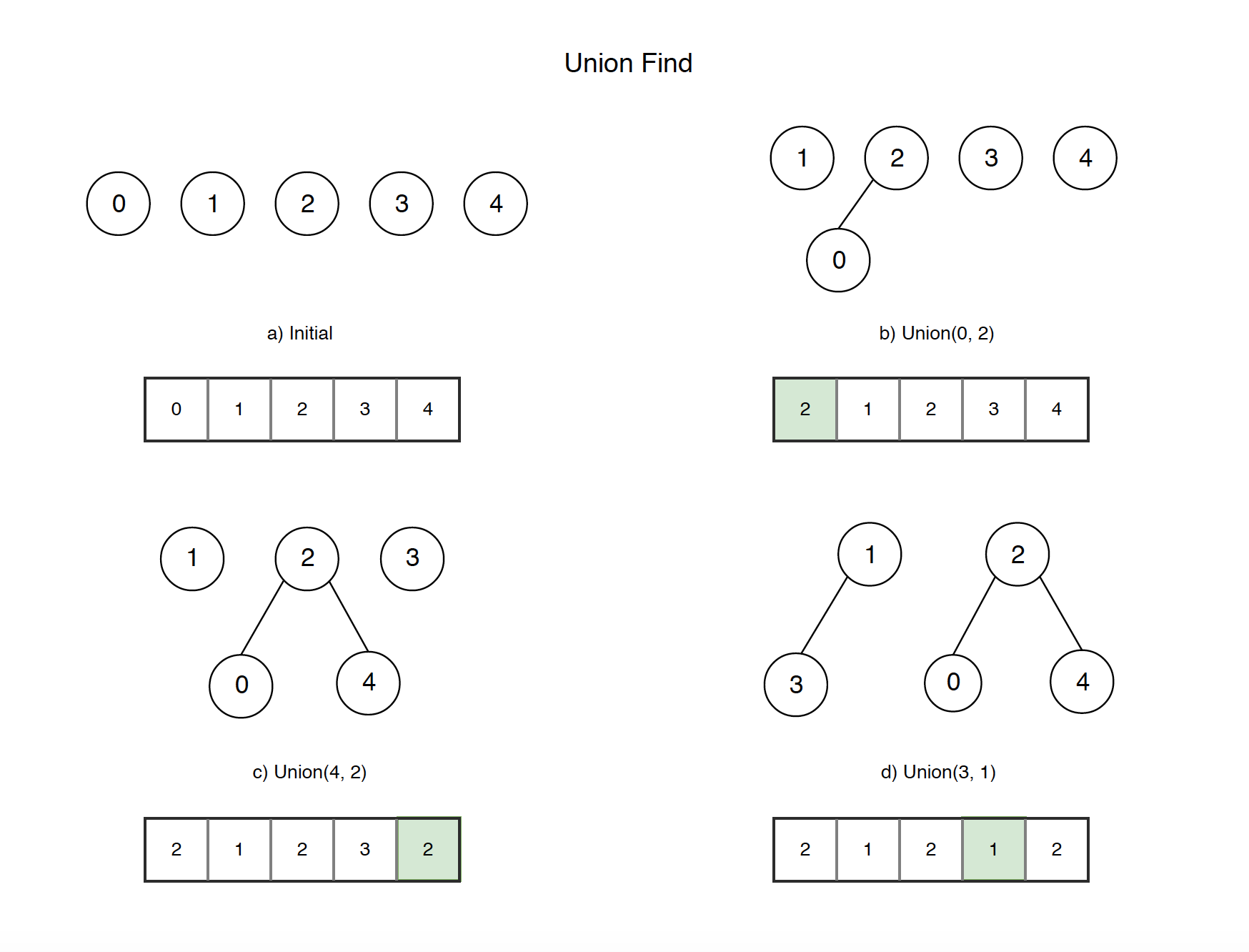
Initialization: We start with N elements, each in its own set. We can use an array of size N, where parent[i] stores the parent of element i. Initially, every element is the root of its own tree, so we set parent[i] = i for all i.
find(i) Operation: To find the representative of element i, we follow the parent pointers. We start at i and move to parent[i], then to parent[parent[i]], and so on, until we reach an element p where parent[p] == p. This element p is the root.
union(i, j) Operation: To unite the sets containing i and j:
a. Find the representative of i: root_i = find(i).
b. Find the representative of j: root_j = find(j).
c. If root_i and root_j are different, merge the sets by setting the parent of one root to the other. For example, parent[root_j] = root_i.

The following resource from cp-algorithms.com provides a concise explanation of this array-based approach and includes the code for a naive implementation.

Disjoint Set Union

This article formalizes the concepts we've discussed and presents a simple implementation.

Please read the introduction and the first two main sections: Start from the beginning and read up to the section on building an efficient data structure. Pay attention to the three core operations defined: make_set, union_sets, and find_set. Continue to the section Build an efficient data structure. This explains the tree-based representation. Finally, read the section Naive implementation. This part shows you the code for the simple find_set and union_sets functions that directly follow the logic we just described.

To see this process in action, the next video from WilliamFiset provides a step-by-step visualization of how a series of union operations modifies the parent array and the corresponding tree structures.

Union Find - Union and Find Operations

This video provides a dynamic walkthrough of the union and find operations.

Watch the following segments: This long segment demonstrates a sequence of union operations. Observe how for each union(x, y), the algorithm first finds the roots of x and y and then connects one root to the other by updating a single value in the parent array. The summary at the end clearly recaps the logic for both the find and union operations.

The image below shows the state of the data structure after a few union operations. Notice how the array values directly reflect the parent pointers in the tree diagrams.

This diagram shows the evolution of a Union-Find structure. Initially, every element is its own parent (a). After `Union(0, 2)`, node 0's parent becomes 2, reflected in the array `parent[0] = 2` (b). Subsequent unions further build up the trees (c, d).

The Problem with the Naive Approach

This simple implementation works, but it has a potential performance issue. If we are not careful about how we merge trees, we can end up creating very tall, stringy trees that look more like linked lists. For example, if we always make the second set's root the child of the first, a sequence like union(0, 1), union(1, 2), union(2, 3) would create a chain 3 -> 2 -> 1 -> 0.

In such a case, calling find(3) would require traversing the entire chain, taking O(N) time, where N is the number of elements. This is inefficient, and it's a problem we will solve in the next lesson.

Conclusion

In this lesson, we introduced the Union-Find data structure and its fundamental purpose: to efficiently manage a collection of disjoint sets.

Key Takeaways:

Purpose: Union-Find is used to track elements partitioned into non-overlapping sets, with common applications in graph connectivity problems.
Core Operations: The two main operations are find (to identify an element's set by finding its representative) and union (to merge two sets).
Representation: The sets are conceptually modeled as a forest of trees. Each tree is a set, and its root is the set's representative.
Implementation: A simple and effective way to implement this is with a parent array, where parent[i] points to the parent of element i. A root node is an element p such that parent[p] == p.
Naive Approach: The basic implementation of union can lead to tall, unbalanced trees, making the find operation slow in the worst case.

You now have a solid conceptual and practical foundation for what Union-Find is and how it works. In our next lesson, we will address the performance issues of the naive approach by introducing two powerful optimizations: path compression and union by rank/size. These techniques will dramatically improve the efficiency of the operations, making Union-Find one of the fastest data structures available for its class of problems.