Trie Complexity Analysis

Welcome to the final lesson in our module on Tries. Over the past few lessons, you've built a solid foundation: you learned the fundamental structure of a Trie, how to implement its core operations, how to leverage it for optimizing complex backtracking searches like in Word Search II, and even how to handle advanced wildcard matching.

Today, we will consolidate this knowledge by formally analyzing the time and space complexity of these common Trie operations. For someone preparing for technical interviews and aiming for a deep, "neat" understanding of data structures, being able to articulate these performance characteristics is just as important as writing the code itself. We will break down the complexity of insert, search, and startsWith, and discuss the critical trade-offs that determine when a Trie is the superior choice over a structure like a hash map.

Time Complexity: The Power of Prefix Traversal

Let's begin by analyzing the time it takes to perform the three fundamental operations on a Trie. The key insight for all three is that the work required is proportional only to the length of the string involved, not the total number of strings stored in the Trie.

Let's define our variables:

• $L$ will be the length of the word or prefix we are working with.
• $N$ will be the total number of words stored in the Trie.
• $K$ will be the size of the alphabet (e.g., 26 for lowercase English letters).

For insert(word), search(word), and startsWith(prefix), the algorithm is the same: traverse the Trie from the root, one character at a time. At each node, we need to find the child corresponding to the current character. Assuming we implement the children pointers using a fixed-size array (as is common in competitive programming) or a hash map, this lookup is an $O(1)$ operation on average.

Since we perform one such traversal for each of the $L$ characters in the string, the total time complexity for all three standard operations is $O(L)$.

The following resource provides a clear walkthrough of these operations and their complexities.

This $O(L)$ performance is a significant advantage. If you were to store $N$ strings in a simple list and check for a prefix, you might have to inspect every string, leading to a much slower $O(N\cdot L)$ complexity.

For a visual and auditory explanation, the following video walks through the insert and search logic, confirming the time complexity at the end of each segment.

Space Complexity: A Tale of Two Metrics

Analyzing space complexity for Tries requires looking at two different aspects: the total space occupied by the data structure and the auxiliary space used by a single operation.

1. Auxiliary Space of Operations

This refers to the extra memory an operation needs while it runs, not including the storage of the Trie itself.

• search(word) and startsWith(prefix): These operations are purely read-only. They traverse existing nodes using a single pointer. Therefore, their auxiliary space complexity is $O(1)$.
• insert(word): This operation might create new nodes. In the worst-case scenario, if you insert a word of length $L$ that shares no prefix with any existing word, you will create $L$ new TrieNode objects. Thus, the auxiliary space complexity for insertion is $O(L)$.

The GeeksforGeeks article you just read highlights this distinction, and the next video provides an exceptionally clear and concise summary.

2. Total Space of the Trie

The total space consumed by the Trie itself depends heavily on its implementation—specifically, how each node stores its children. This is a classic time-space trade-off.

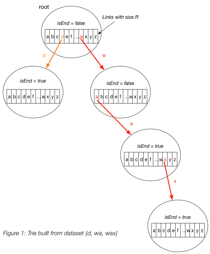
The video segment below discusses this trade-off in detail, comparing four different implementation strategies for the children pointers.

As the video explains:

• Array of size K: Each node holds an array of size $K$. This gives $O(1)$ time to access any child but can be very wasteful. The total space is O(\text{num_nodes} \cdot K). For a large alphabet and a sparse trie (where most nodes have few children), this leads to a lot of unused null pointers.
• Hash Map: Each node holds a hash map mapping characters to child nodes. This is much more space-efficient, as you only store pointers for children that actually exist. The total space is proportional to the total number of characters in all unique prefixes. However, access time has a slightly higher constant factor than a direct array index, though it's still $O(1)$ on average.

When to Use a Trie: Trie vs. Hash Map

Now we can answer a crucial question: when should you choose a Trie over a simple hash map (or hash set) for storing strings?

Operation	Trie	Hash Map (of strings)
insert(word)	$O(L)$	Average: $O(L)$
search(word)	$O(L)$	Average: $O(L)$
startsWith(prefix)	$O(L)$	$O(N\cdot L)$
Space Complexity	Can be high (O(\text{num_nodes} \cdot K))	Proportional to sum of all string lengths

As the table shows, for single-word insertion and search, the performance is comparable. The Trie's unique advantage lies in prefix-based operations. A hash map is not structured to find all keys starting with a certain prefix efficiently. You would have to iterate through all $N$ keys.

Your experience as an intern might give you context for this. Think of systems like an API gateway routing incoming requests based on URL paths. A path like /api/v1/users/123 can be treated as a string. A Trie can store all valid API routes (e.g., /api/v1/users, /api/v2/products) and perform a longest-prefix match in time proportional to the path length, not the total number of routes in the system.

Complexity of Advanced Operations

Finally, let's briefly recall the complexity of the wildcard search we covered in the last lesson. When searching for a pattern like b.d, the . character forces the algorithm to branch. In the worst case, a search for ... (length $L$) on a Trie with a branching factor of $K$ at each level could explore $O(K^L)$ paths. This exponential time complexity is a critical trade-off for the added flexibility. The space complexity for the recursive wildcard search is $O(L)$ due to the depth of the recursion stack.

Conclusion

You have now completed our deep dive into the Trie data structure. You can not only implement its various functions but also analyze their performance and justify its use over other structures.

Key Takeaways:

• Time Complexity: Standard Trie operations (insert, search, startsWith) are highly efficient, with a time complexity of $O(L)$, where $L$ is the length of the string. This is independent of the number of words in the Trie.
• Space Complexity: The auxiliary space for search/startsWith is $O(1)$, while for insert it is $O(L)$. The total space of the Trie itself presents a time-space trade-off, depending on whether children are stored in a fixed array or a more dynamic structure like a hash map.
• Use Case: A Trie's primary advantage over a hash map is its efficiency in prefix-based searches, making it ideal for applications like autocomplete, IP routing, and API gateways.
• Advanced Operations: More complex operations like wildcard searching can have significantly higher (even exponential) time complexity, which is an important consideration.

In our next module, we will shift gears to an entirely different data structure: the Union-Find (or Disjoint Set Union). It is a remarkably efficient structure designed to solve problems involving connectivity, partitioning, and dynamic grouping of elements.