EM Algorithm for Latent Variable Models

Recommended resources

The freely available resources this lesson will direct you to.

Introduction

In our last lesson, we introduced Gaussian Mixture Models (GMMs) as a powerful probabilistic method for clustering and density estimation. We concluded by highlighting the central challenge in fitting a GMM: maximizing the log-likelihood function is intractable due to the sum over components appearing inside the logarithm. This "log-of-a-sum" problem prevents a simple, closed-form solution. We ended with an intuitive iterative procedure—calculate cluster responsibilities, then update model parameters—and noted this was an instance of a more general algorithm.

This lesson delivers on that promise by formally deriving the Expectation-Maximization (EM) algorithm. You will learn how EM provides a principled, general framework for finding maximum likelihood estimates in models with latent variables. We will begin by formalizing the iterative intuition we developed for GMMs and then build a rigorous mathematical justification from first principles, proving why this two-step process is guaranteed to improve the model's likelihood at each iteration. This derivation is a cornerstone of modern machine learning, applicable far beyond the GMMs we use as our motivating example.

The Problem of Missing Information

The core difficulty in training a GMM stems from a missing piece of information: we don't know which Gaussian component generated each data point. This "component identity" is a latent variable. Let's formalize this.

As we saw, the log-likelihood for a GMM is:

ln p (X ∣ θ) = n = 1 \sum N ln (k = 1 \sum K ϕ_{k} N (x_{n} ∣ μ_{k}, Σ_{k}))

This is the likelihood of the incomplete data $X$ .

Now, imagine we had access to the latent variables $Z$ , where $z_{nk} = 1$ if data point $x_{n}$ came from component $k$ , and 0 otherwise. This would give us the complete data ${X, Z}$ . The complete-data log-likelihood would be:

ln p (X, Z ∣ θ) = n = 1 \sum N k = 1 \sum K z_{nk} {ln ϕ_{k} + ln N (x_{n} ∣ μ_{k}, Σ_{k})}

Notice the crucial difference: the logarithm now acts directly on the Gaussian and the mixing coefficient. The "sum-inside-the-log" problem has vanished. Maximizing this function is straightforward; it decouples into separate, simple maximization problems for each component $k$ , using only the data points assigned to it.

Of course, we don't know $Z$ . This is where the Expectation-Maximization strategy comes in. It suggests an iterative process to deal with this missing information.

The "E" Step (Expectation): Since we don't know the exact values of the latent variables $Z$ , we use our current parameter estimates ( $θ^{old}$ ) to compute their expected values. The expectation of the indicator variable $z_{nk}$ is simply the posterior probability that point $x_{n}$ belongs to component $k$ , which is the responsibility $γ (z_{nk})$ . We use these responsibilities to compute the expectation of the complete-data log-likelihood. This expected value is called the auxiliary function, $Q (θ, θ^{old})$ .
The "M" Step (Maximization): We maximize this auxiliary function $Q (θ, θ^{old})$ with respect to the parameters $θ$ to find our updated estimates, $θ^{new}$ . Because the $Q$ function has the friendly, decoupled form of the complete-data log-likelihood, this maximization step is tractable.

A Concrete Analogy: The Mystery Coins

Before diving into the general derivation, let's build intuition with a simpler example. Imagine a game with two different biased coins, A and B. We perform 5 experiments. In each, we secretly pick one of the coins, toss it 10 times, and record the sequence of heads (H) and tails (T). Our goal is to estimate the probability of heads for each coin, $θ^_{A}$ and $θ^_{B}$ .

This image contrasts estimating coin biases when the source coin for each sequence is known (Maximum Likelihood) versus unknown (Expectation-Maximization). Source: Stack Exchange.

Case A: Maximum Likelihood (Complete Data)
In the top panel, we are told which coin was used for each of the 5 sequences. The latent variable (the coin's identity) is observed. The problem is simple. To find $θ^_{A}$ , we just count the total heads and tails from the sequences generated by coin A (24H, 6T) and compute the MLE: $θ^_{A} = 24/ (24 + 6) = 0.80$ . We do the same for coin B. This is analogous to maximizing the complete-data log-likelihood.

Case B: Expectation-Maximization (Incomplete Data)
In the bottom panel, we are only given the 5 sequences; we don't know which coin generated which. This is a latent variable problem. We use EM:

Initialization (Step 1): We start with a random guess for the parameters, say $θ^_{A}^{(0)} = 0.60$ and $θ^_{B}^{(0)} = 0.50$ .
E-Step (Step 2): For each sequence, we calculate the probability that it came from coin A versus coin B, given our current parameter guesses. For the first sequence (HTT...), the probability of observing it if it came from coin A is $(0.6)^{5} (0.4)^{5}$ , while from coin B it's $(0.5)^{5} (0.5)^{5}$ . By normalizing these probabilities, we might find there's a 45% chance it came from A and a 55% chance it came from B. We do this for all 5 sequences. These are our "responsibilities."
M-Step (Step 3): Now, we re-estimate the parameters. For $θ^_{A}$ , we calculate the expected number of heads and tails assigned to it. If the first sequence has a 45% chance of being from A, we credit 45% of its heads and tails (i.e., $0.45 \times 5 H$ and $0.45 \times 5 T$ ) to coin A's tally. We sum these expected counts over all 5 sequences to get a total expected count (e.g., 21.3 H and 8.6 T for coin A). We then update our estimate: $θ^_{A}^{(1)} = 21.3/ (21.3 + 8.6) \approx 0.71$ .
Iteration (Step 4): We repeat the E-step and M-step with our new estimates ( $θ^_{A}^{(1)} = 0.71, θ^_{B}^{(1)} = 0.58$ ). The algorithm continues until the parameter estimates converge, in this case to values close to the true ones used in Case A.

This iterative "guessing" and "re-estimating" is the essence of EM. Now let's prove why this process is mathematically sound.

The General Derivation of EM

The key question is: why does this iterative process of maximizing the expected complete-data log-likelihood lead to a maximum of the actual incomplete-data log-likelihood we care about? To answer this, we'll construct a lower bound on the log-likelihood and show that EM is a procedure for iteratively maximizing this bound.

This derivation, while abstract, is one of the most elegant results in machine learning. We will first walk through the concepts in a lecture from Stanford and then provide the full text derivation for your detailed study.

The derivation hinges on a fundamental result from information theory and statistics: Jensen's Inequality. For a concave function like the logarithm, Jensen's inequality states that the function of an expectation is greater than or equal to the expectation of the function: $lo g (E [X]) \geq E [lo g (X)]$ .

We can use this to establish a lower bound on our log-likelihood function $ln p (X ∣ θ)$ .

Lecture 14 - Expectation-Maximization Algorithms | Stanford CS229: Machine Learning (Autumn 2018)

This video segment from Andrew Ng's Stanford CS229 course provides a clear, step-by-step derivation of the EM algorithm. It masterfully uses visual aids to explain the core concepts.

Please watch from the derivation section. Pay close attention to these key parts: Jensen's Inequality: The visual explanation of why f(E[x]) <= E[f(x)] for convex functions (and the reverse for concave functions like log). Constructing the Lower Bound: Follow the algebraic steps where an arbitrary distribution Q(z) is introduced (multiplied and divided) and Jensen's inequality is applied to push the log inside the expectation, creating a lower bound on the true log-likelihood. The Visual Intuition: Keep the mental model of the blue log-likelihood curve and the green lower-bound curve that EM constructs and maximizes in each step.

As the video demonstrates, for any distribution $q (Z)$ over the latent variables, we can decompose the log-likelihood as:

ln p (X ∣ θ) = L (q, θ) + KL (q (Z) ∣∣ p (Z ∣ X, θ))

where:

$L (q, θ) = \sum_{Z} q (Z) lo g \frac{p ( X , Z ∣ θ )}{q ( Z )}$ is the Evidence Lower Bound (ELBO).
$KL (\cdot ∣∣ \cdot)$ is the Kullback-Leibler divergence, which is always non-negative ( $\geq 0$ ).

Since the KL divergence is non-negative, we have $ln p (X ∣ θ) \geq L (q, θ)$ . The ELBO is indeed a lower bound on the evidence (the log-likelihood).

EM as Coordinate Ascent

The EM algorithm can be viewed as performing coordinate ascent on the ELBO, $L (q, θ)$ , alternately optimizing with respect to $q$ and $θ$ .

E-Step: Maximize $L (q, θ)$ with respect to $q$
With $θ$ held fixed at its old value $θ^{old}$ , we maximize the ELBO with respect to the distribution $q (Z)$ . From the decomposition above, this is equivalent to making the KL divergence term equal to zero. This happens if and only if we set $q (Z)$ to be exactly the posterior distribution of the latent variables:

q (Z) = p (Z ∣ X, θ^{old})

This is precisely the E-step: we calculate the posterior distribution over the latent variables (for GMMs, this is the set of all responsibilities). At this point, the lower bound $L$ is "tight"—it touches the true log-likelihood curve at the point $θ^{old}$ .

M-Step: Maximize $L (q, θ)$ with respect to $θ$
With $q (Z)$ held fixed at $p (Z ∣ X, θ^{old})$ , we maximize the ELBO with respect to the parameters $θ$ . It can be shown that maximizing $L (q, θ)$ is equivalent to maximizing the expected complete-data log-likelihood, $Q (θ, θ^{old})$ , which we defined earlier.

θ^{new} = ar g θ max L (q, θ) = ar g θ max Q (θ, θ^{old})

Since we are maximizing a lower bound on the true log-likelihood, this step guarantees that the log-likelihood will not decrease.

This two-step process—finding the best lower bound at the current parameter setting, then moving to the maximum of that bound—ensures that we are always climbing the log-likelihood surface.

To solidify your understanding of this coordinate ascent process and the role of KL-divergence, the following video provides an excellent and complementary perspective.

27. EM Algorithm for Latent Variable Models

This lecture from the "Foundations of Machine Learning" series at Bloomberg provides a very clear explanation of EM as a coordinate ascent process on the ELBO.

Please watch the segment from this explanation. Focus on the decomposition of the log-likelihood into the ELBO and the KL-divergence, and how the E-step is elegantly framed as choosing a Q to minimize this KL divergence to zero.

For a complete, rigorous treatment that you can read through at your own pace, Chapter 9 of Christopher Bishop's Pattern Recognition and Machine Learning is the definitive source.

Mixture Models and EM

This text provides the formal mathematical foundation for the EM algorithm, which will be highly valuable given your background.

First, read the section "An Alternative View of EM" to see the general definition of the Q function as the expected complete-data log likelihood. Start from this discussion and follow it to the end of the section. Next, for the complete proof, read the section "The EM Algorithm in General." It starts by defining the lower bound \mathcal{L}(q, \theta) and uses the KL-divergence to show that the E-step and M-step together guarantee an increase in the log-likelihood. This is the theoretical heart of the algorithm.

Visualizing Convergence

With the theory in hand, we can now appreciate what happens in practice. The EM algorithm iteratively refines the parameters of the GMM, causing the Gaussian components to move and reshape themselves to best fit the clusters in the data. Each step in this process corresponds to one cycle of the E-step and M-step, which we've just proven corresponds to an increase in the model's log-likelihood.

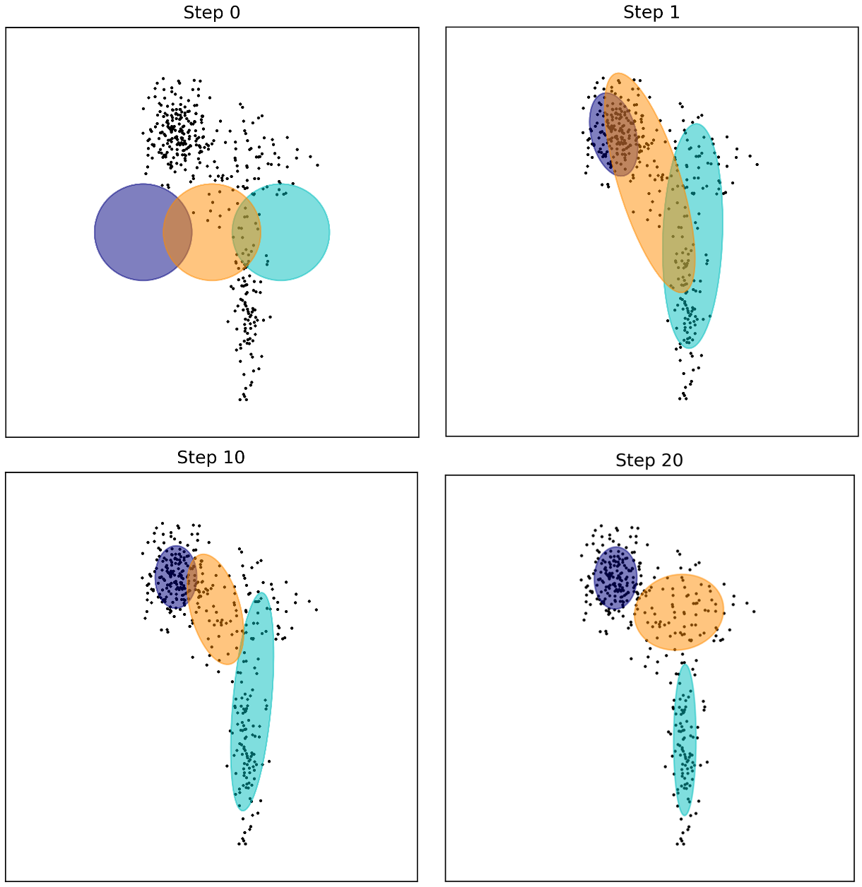
An illustration of the EM algorithm fitting a Gaussian Mixture Model with three components to a dataset. The ellipses represent the one-standard-deviation contours of the Gaussians. The algorithm starts with a random initialization (Step 0) and converges to a good fit of the underlying clusters over 20 iterations.

As you can see, the process begins with poorly placed, spherical Gaussians. Through successive iterations, the algorithm moves the means, adjusts the covariances (allowing the ellipses to rotate and stretch), and refines the mixing weights until the components accurately capture the three distinct groups in the data.

Conclusion

In this lesson, we have constructed the Expectation-Maximization algorithm from the ground up. We began with the practical problem of fitting a GMM and the intuition of an iterative solution, then formalized it into a general and powerful statistical tool for any model with latent variables.

Here are the key takeaways from our derivation:

Latent Variables: The intractability of maximizing the log-likelihood in models like GMMs is due to unobserved (latent) variables.
Complete vs. Incomplete Data: If the latent variables were known (complete data), MLE would be easy. EM is a strategy to handle the real-world incomplete data case.
The ELBO: We can construct a function, the Evidence Lower Bound (ELBO), which is always less than or equal to the true log-likelihood.
Coordinate Ascent: The EM algorithm is a two-stage process that iteratively maximizes this lower bound. The E-step finds the best bound at the current parameter values, and the M-step moves to the maximum of that bound. This guarantees that each EM iteration improves (or maintains) the log-likelihood of the model.
Generality: Although we used GMMs as our guide, the EM derivation is completely general and applies to a vast range of problems involving missing data or latent structure, including Hidden Markov Models (HMMs), Factor Analysis, and some Bayesian networks.

In our next lesson, we will explore another popular unsupervised learning technique, t-SNE, which tackles a different problem: visualizing high-dimensional data in a low-dimensional space while preserving local structure.