Gaussian Mixture Models vs. K-means: A Probabilistic Approach to Density Estimation

Recommended resources

The freely available resources this lesson will direct you to.

Density Estimation with Gaussian Mixture Models (GMM) and Empirical Priorswww.youtube.com
Stanford CS229: Machine Learning | Summer 2019 | Lecture 16 - K-means, GMM, and EMwww.youtube.com
[PDF] Mixture Models - Statistics & Data Sciencewww.stat.cmu.edu
Gaussian Mixture Models and Expectation Maximization ...users.cs.duke.edu

Introduction

In our recent lessons on unsupervised learning, we first covered K-means for clustering and then explored PCA for dimensionality reduction. We saw how PCA uses the data's covariance structure to find a lower-dimensional representation, and you learned how to select the number of components based on explained variance. Now, we return to the theme of clustering but from a more powerful, probabilistic standpoint.

This lesson introduces Gaussian Mixture Models (GMMs). You will learn how GMMs represent a dataset not as a collection of hard, geometric clusters like in K-means, but as a mixture of several Gaussian distributions. We will explore how this probabilistic foundation allows GMMs to perform both "soft" clustering and density estimation, offering a much more flexible and informative view of the data's underlying structure. The central goal is to understand the GMM framework and contrast its probabilistic approach with the deterministic assignments of K-means. This will set the stage for our next lesson, where we will derive the algorithm used to train these models.

The Limitations of a Hard-Clustering Approach

Let's begin by revisiting the K-means algorithm. Its core principle is hard assignment: each data point is assigned to exactly one cluster, the one with the nearest centroid. This approach is intuitive and computationally efficient, but it relies on strong, often implicit, assumptions about the data's structure.

Specifically, by using Euclidean distance to measure closeness to a centroid, K-means inherently favors clusters that are:

Spherical: The distance metric doesn't account for correlations between features, so it looks for ball-shaped groups.
Equally Sized: The algorithm has no built-in mechanism to handle clusters of different variances or densities.

When these assumptions are violated, K-means can produce counter-intuitive or misleading results.

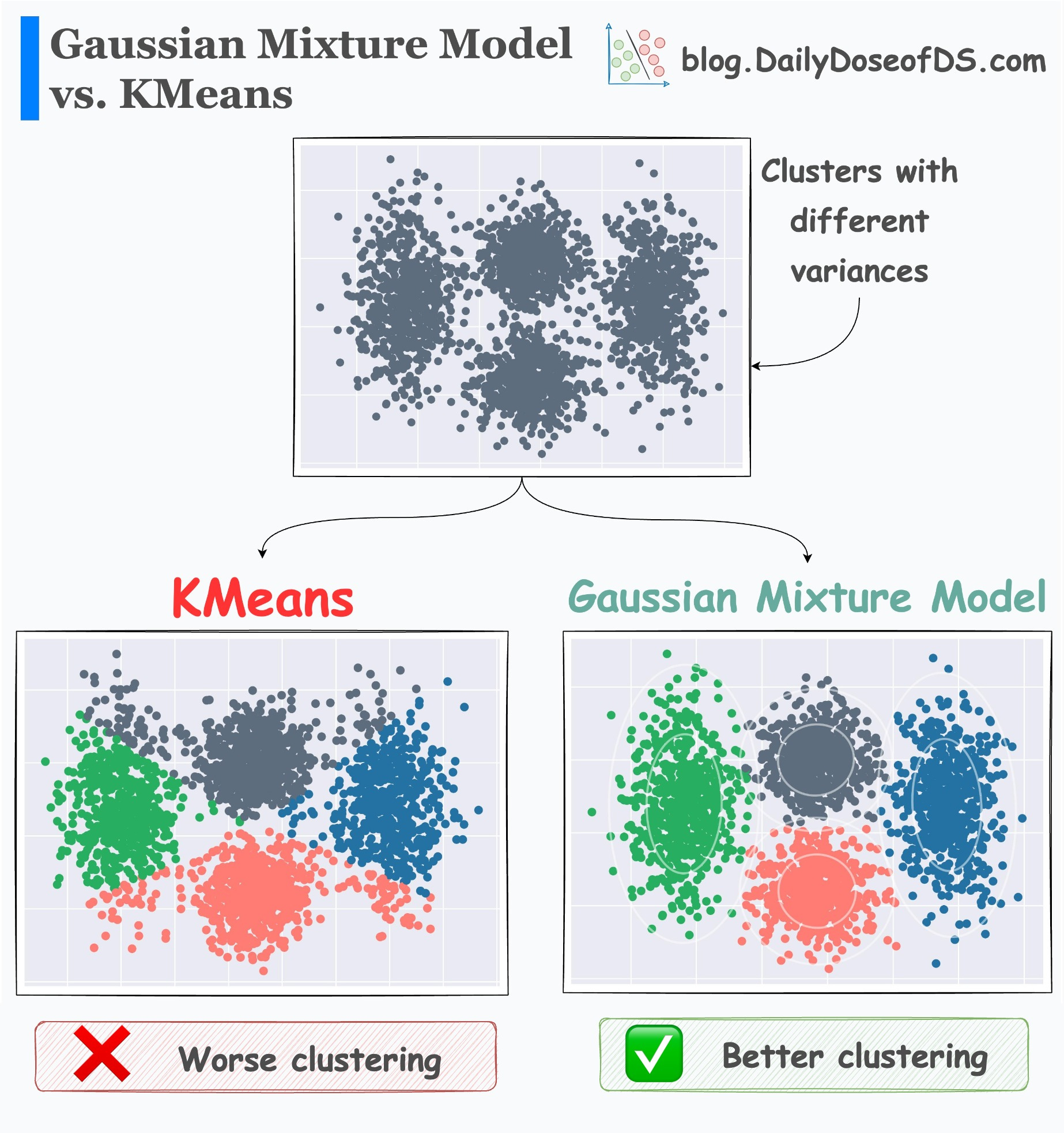
This image shows data generated from several clusters with different variances. K-means struggles to correctly identify the boundaries, splitting parts of the same natural group. GMM, which we will study, correctly models the clusters by accounting for their different shapes and sizes.

Here, the clusters are elongated and overlapping. K-means, seeking spherical groups, incorrectly partitions the data. The Gaussian Mixture model on the left correctly identifies the elliptical structure of the clusters.

These examples highlight the need for a more flexible model—one that can capture varied cluster shapes and express uncertainty in cluster assignments.

A Probabilistic Model of Data: The Gaussian Mixture Model

Instead of thinking about clusters as geometric regions, what if we adopted a generative perspective? We can assume that our data was generated from a combination of several underlying probability distributions. This is the core idea behind Gaussian Mixture Models (GMMs).

A GMM assumes that the data is generated from a mixture of $K$ different Gaussian distributions. The generative process for a single data point $x$ is as follows:

First, choose a component (a specific Gaussian) $k \in {1, \dots, K}$ . This choice is governed by a set of mixing weights $ϕ_{k}$ , where $ϕ_{k}$ is the probability of choosing component $k$ , and $\sum_{k = 1}^{K} ϕ_{k} = 1$ . This choice can be represented by a latent categorical variable $z$ .
Once a component $k$ is chosen, sample the data point $x$ from that component's Gaussian distribution, $N (x ∣ μ_{k}, Σ_{k})$ , which is defined by its own mean $μ_{k}$ and covariance matrix $Σ_{k}$ .

This process leads to a model whose probability density function (PDF) is a weighted sum of individual Gaussian densities:

p (x ∣ θ) = k = 1 \sum K ϕ_{k} N (x ∣ μ_{k}, Σ_{k})

Here, $θ = {ϕ_{k}, μ_{k}, Σ_{k}}_{k = 1}^{K}$ represents the full set of model parameters.

This lecture from Stanford Online provides an excellent introduction to the concepts of density estimation and the GMM framework.

Stanford CS229: Machine Learning | Summer 2019 | Lecture 16 - K-means, GMM, and EM

The lecturer, Anand Mamgain, provides a clear transition from clustering to density estimation and motivates the need for GMMs.

Please watch two segments: First, watch from the beginning up to the introduction of K-means, focusing on the discussion of unsupervised learning and clustering (introduction). Then, skip the K-means review and watch the section that introduces density estimation and the Gaussian Mixture Model (Density Estimation & GMM). Pay close attention to the aircraft part manufacturing example for anomaly detection, which is a key application of density estimation. Also, focus on the formal description of the GMM generative process involving the latent variable z.

GMM: Two Sides of the Same Coin

The GMM formulation provides two powerful capabilities: density estimation and soft clustering.

1. Density Estimation
The primary interpretation of a GMM is as a density estimator. The equation $p (x) = \sum ϕ_{k} N (x ∣ μ_{k}, Σ_{k})$ provides a smooth, continuous probability density function that approximates the true distribution of the data. This is extremely powerful. Once we have this function, we can evaluate the probability density of any point, including new, unseen data. This is the basis for tasks like anomaly detection: points that fall in low-density regions of the model are flagged as anomalies. This video from Steve Brunton gives a nice overview of this idea.

Density Estimation with Gaussian Mixture Models (GMM) and Empirical Priors

This video discusses density estimation in a broader context and provides a clear conceptual picture of what a GMM is doing.

Please watch the segment from Gaussian Mixture Models. Notice how he visualizes the GMM as a sum of a few Gaussians that approximate a more complex underlying distribution in both 1D and 2D.

2. Soft Clustering
While K-means performs a hard assignment, GMMs provide a soft assignment. For any given data point $x_{i}$ , instead of assigning it to a single cluster, we can calculate the posterior probability that it belongs to each component $k$ . Using Bayes' theorem, this responsibility, or soft assignment, is given by:

γ (z_{ik}) = p (z_{i} = k ∣ x_{i}, θ) = \frac{p ( z _{i} = k ∣ θ ) p ( x _{i} ∣ z _{i} = k , θ )}{p ( x _{i} ∣ θ )} = \frac{ϕ _{k} N ( x _{i} ∣ μ _{k} , Σ _{k} )}{\sum _{j = 1}^{K} ϕ _{j} N ( x _{i} ∣ μ _{j} , Σ _{j} )}

The value $γ (z_{ik})$ is the "responsibility" that component $k$ takes for explaining data point $i$ . For each point $i$ , we get a vector of probabilities ${γ (z_{i 1}), γ (z_{i 2}), \dots, γ (z_{i K})}$ that sum to 1. This is a much richer representation than a single cluster label. Points deep inside one cluster will have a responsibility close to 1 for that cluster and close to 0 for others. Points in overlapping regions will have divided responsibilities.

The Contrast with K-means

We can now draw a formal contrast between GMM and K-means, which directly addresses our learning outcome.

Feature	K-means	Gaussian Mixture Model (GMM)
Model Type	Non-probabilistic, geometric	Probabilistic, generative
Cluster Assignment	Hard: Each point belongs to one cluster.	Soft: Each point has a probability of belonging to each cluster (responsibilities).
Cluster Shape	Assumes spherical clusters of equal size.	Can model flexible, elliptical clusters via covariance matrices $Σ_{k}$ .
Output	Cluster labels and centroids ( $μ_{k}$ ).	Full probability distribution parameters ( $ϕ_{k}, μ_{k}, Σ_{k}$ ) for density estimation and new data generation.
Objective	Minimize within-cluster sum of squares (distortion).	Maximize the log-likelihood of the observed data.

This document from CMU provides a succinct, theoretical discussion on this contrast.

[PDF] Mixture Models - Statistics & Data Science

This document gives a formal statistical treatment of mixture models.

Please read the section on "Probabilistic Clustering." Focus on the paragraph that begins here. It highlights the predictive power of probabilistic models like GMMs compared to non-probabilistic methods like K-means.

The Estimation Problem: A Glimpse of Expectation-Maximization

We have defined the GMM, but how do we find its parameters $θ = {ϕ_{k}, μ_{k}, Σ_{k}}_{k = 1}^{K}$ from the data? The standard approach in statistics is Maximum Likelihood Estimation (MLE). We want to find the parameters $θ$ that maximize the log-likelihood of our observed data $X = {x_{1}, \dots, x_{n}}$ .

L (θ) = lo g p (X ∣ θ) = i = 1 \sum n lo g p (x_{i} ∣ θ) = i = 1 \sum n lo g (k = 1 \sum K ϕ_{k} N (x_{i} ∣ μ_{k}, Σ_{k}))

The problem, as your computer science background might lead you to spot, is the log of a sum. This structure prevents a closed-form analytical solution. If the sum were inside the logarithm, we could solve it easily. But with the sum outside, taking derivatives and setting them to zero becomes intractable.

This is where the latent variables $z_{i}$ become conceptually useful. If we knew which Gaussian generated each point (i.e., if we knew the $z_{i}$ ), the problem would be simple. We could just partition the data and estimate the mean and covariance for each group. This leads to a chicken-and-egg problem:

If we knew the parameters $θ$ , we could compute the cluster responsibilities $γ (z_{ik})$ .
If we knew the cluster responsibilities $γ (z_{ik})$ , we could update the parameters $θ$ .

This circular logic strongly suggests an iterative algorithm. We can:

Initialize the parameters $θ$ (e.g., randomly or using K-means).
Repeat until convergence:
a. Expectation (E-step): Given the current parameters, calculate the responsibilities $γ (z_{ik})$ for each point. This is our "expectation" of which cluster each point belongs to.
b. Maximization (M-step): Given the current responsibilities, update the parameters $θ$ to maximize the likelihood. This involves calculating new weighted means, covariances, and mixing coefficients.

The following notes provide the update equations derived from this logic.

Gaussian Mixture Models and Expectation Maximization ...

These notes from Duke University provide a clear mathematical derivation for the GMM update rules within the EM framework.

Please read the sections detailing the E-step and M-step specifically for GMM. Start at the E-step explanation to see how the responsibilities (\gamma_{ik}) are calculated. Then, read the M-step derivation to see how those responsibilities are used as weights to update the parameters \mu_k, \Sigma_k, w_k. You can skim the Lagrangian derivation for the weights w_k for now; the key insight is the weighted average form of the updates for the mean and covariance.

This intuitive iterative process is an instance of a powerful and general algorithm called Expectation-Maximization (EM), which we will derive from first principles in our next lesson.

Conclusion

In this lesson, we have moved from the geometric world of K-means to the probabilistic framework of Gaussian Mixture Models. You now understand that GMMs model data as a mixture of Gaussian distributions, which provides a principled way to handle non-spherical clusters and uncertainty in assignments.

Here are the key takeaways:

Probabilistic Model: GMMs are generative models that define a probability density over the data space, useful for density estimation and anomaly detection.
Soft Clustering: Unlike K-means' hard assignments, GMMs produce "soft" assignments (responsibilities), quantifying the probability that a data point belongs to each cluster.
Flexibility: GMMs can capture elliptical clusters with varying sizes and orientations through their covariance matrices, making them far more flexible than K-means.
Estimation Challenge: Finding the parameters of a GMM via Maximum Likelihood Estimation is complicated by the "log-of-a-sum" problem, which necessitates an iterative approach.

In our next lesson, we will formalize this iterative solution. We will derive the Expectation-Maximization (EM) algorithm as a general method for performing MLE in models with latent variables, using GMMs as our primary motivating example.