WKB Wavefunction and Connection Formulae

Hello! Welcome to our next lesson.

In our previous lessons, we explored various approximation methods for time-dependent Hamiltonians, culminating with the sudden approximation for very rapid changes. Now, we shift our focus back to the time-independent Schrödinger equation, but for cases where the potential $V(x)$ is too complex to allow for an exact solution.

This brings us to the WKB (Wentzel-Kramers-Brillouin) approximation, a powerful semi-classical method. The core idea is to find approximate solutions in regions where the potential varies slowly compared to the particle's de Broglie wavelength. Your background in classical mechanics will be helpful here, as we'll see many classical concepts re-emerge.

Today, our goal is to derive the WKB wavefunction for one-dimensional systems and then learn how to apply the crucial connection formulae at classical turning points, where the standard WKB approximation breaks down.

1. The Semi-Classical Approach and the WKB Wavefunction

We begin with the one-dimensional time-independent Schrödinger equation (TISE):
$-\frac{{\hslash }^2}{2m}\frac{d^2\psi }{d{x}^2}+V(x)\psi (x)=E\psi (x)$
Rearranging this gives:
$\frac{d^2\psi }{d{x}^2}=-\frac{2m}{{\hslash }^2}(E-V(x))\psi (x)=-\frac{p(x{)}^2}{{\hslash }^2}\psi (x)$
Here, we've defined the position-dependent classical momentum $p(x)=\sqrt{2m(E-V(x))}$.

If $V(x)$ were constant, $p(x)$ would be a constant $p$, and the solutions would be simple plane waves $\psi (x)=e^{\pm ipx/\hslash }$. The WKB approximation assumes that if $V(x)$ varies slowly, the solution should locally resemble a plane wave, but with an amplitude and phase that also vary slowly with position.

To formalize this, we use the ansatz:
$\psi (x)=e^{iS(x)/\hslash }$
where $S(x)$ is a complex function. The imaginary part of $S(x)$ will account for changes in the amplitude of $\psi (x)$. Substituting this into the TISE yields a nonlinear differential equation for $S(x)$:
$(S^{\prime }(x){)}^2-i\hslash S^{\prime \prime }(x)=p(x{)}^2$
This is an exact equation, but it's harder to solve than the original TISE. The breakthrough comes from treating $\hslash$ as a small parameter and performing a series expansion for $S(x)$, known as a semi-classical expansion:
$S(x)=S_0(x)+\hslash S_1(x)+{\hslash }^2{S}_2(x)+\dots$

To see how this works and leads to the final WKB wavefunction, let's turn to a couple of excellent resources.

For a dynamic walkthrough of the same derivation, you might find this video helpful.

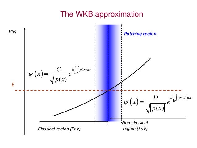
By keeping terms up to $\mathcal{O}(\hslash )$, we arrive at the WKB approximate wavefunction. In the classically allowed region where $E>V(x)$ and $p(x)$ is real, the general solution is a superposition of waves moving left and right:
${\psi }_{WKB}(x)\approx \frac{1}{\sqrt{p(x)}}\left(A{e}^{\frac{i}{\hslash }{\int }^{x}p(x^{\prime })d{x}^{\prime }}+B{e}^{-\frac{i}{\hslash }{\int }^{x}p(x^{\prime })d{x}^{\prime }}\right)$
In the classically forbidden region where $E<V(x)$, the momentum becomes imaginary. We define $\kappa (x)=\sqrt{2m(V(x)-E)}$, so $p(x)=i\kappa (x)$. The wavefunction becomes a combination of exponentially growing and decaying terms:
${\psi }_{WKB}(x)\approx \frac{1}{\sqrt{\kappa (x)}}\left(C{e}^{\frac{1}{\hslash }{\int }^x\kappa (x^{\prime })d{x}^{\prime }}+D{e}^{-\frac{1}{\hslash }{\int }^x\kappa (x^{\prime })d{x}^{\prime }}\right)$

Notice the amplitude factor $1/\sqrt{p(x)}$. This has a nice physical interpretation: the probability of finding a particle, $|\psi {|}^2\propto 1/p(x)$, is inversely proportional to its classical momentum (and thus its speed). This is intuitive—the faster the particle moves, the less time it spends at any given point.

2. Breakdown at Classical Turning Points

The WKB approximation is based on the potential varying slowly. The condition for its validity can be expressed as:
$\left|\frac{d\lambda }{dx}\right|\ll 1$
where $\lambda (x)=2\pi \hslash /p(x)$ is the local de Broglie wavelength. This means the wavelength should not change much over a distance of one wavelength.

Now, consider a classical turning point, a location $x_t$ where the total energy equals the potential energy, $E=V(x_t)$.
At this point, the classical momentum $p(x_t)=0$, and the de Broglie wavelength $\lambda (x_t)$ becomes infinite. The validity condition is catastrophically violated. Furthermore, the WKB wavefunction itself diverges due to the $1/\sqrt{p(x)}$ factor.

The WKB approximation fails near turning points. We need a way to connect the oscillatory solution in the allowed region to the exponential solution in the forbidden region across this problematic point.

3. Connection Formulae via the Airy Function

The strategy to bridge the gap is to solve the Schrödinger equation exactly in the small region around the turning point and then "match" this solution to the WKB solutions on either side.

1. Linearize the Potential: Near a turning point $x_t$, we can approximate the potential with a Taylor expansion:
   $V(x)\approx V(x_t)+V^{\prime }(x_t)(x-x_t)=E+C(x-x_t)$
   where $C=V^{\prime }(x_t)$ is a constant. We assume $V^{\prime }(x_t)\ne 0$.

2. The Airy Equation: With this linear potential, the TISE becomes:
   $-\frac{{\hslash }^2}{2m}\frac{d^2\psi }{d{x}^2}+C(x-x_t)\psi =0$
   By making a linear change of variables, $u={\left(\frac{2mC}{{\hslash }^2}\right)}^{1/3}(x-x_t)$, this equation transforms into the famous Airy equation:
   $\frac{d^2\psi }{d{u}^2}-u\psi =0$

3. The Airy Function and its Asymptotics: The physically acceptable solution to this equation (one that doesn't blow up in the forbidden region) is the Airy function, Ai($u$). You can see its form in Figure 66 of Tong's notes (LINK). Its key feature is its asymptotic behavior:

   • For $u\gg 0$ (deep in the forbidden region):
     $\text{Ai}(u)\sim \frac{1}{2\sqrt{\pi }{u}^{1/4}}{e}^{-\frac{2}{3}{u}^{3/2}}(\text{Exponentially decaying})$
   • For $u\ll 0$ (deep in the allowed region):
     $\text{Ai}(u)\sim \frac{1}{\sqrt{\pi }(-u{)}^{1/4}}\sin \left(\frac{2}{3}(-u{)}^{3/2}+\frac{\pi }{4}\right)(\text{Oscillatory})$

4. Matching and the Connection Formulae: The final step is to match these asymptotic forms of the exact Airy function solution to our WKB approximate solutions. This matching process establishes a rigorous connection between the coefficients and phases of the wavefunctions on either side of the turning point.

A detailed derivation of this matching is quite instructive.

The result of this matching procedure gives us the celebrated WKB connection formulae.

Let's consider a turning point $x_t$ where the potential is rising, so the classically allowed region is to the left ($x<x_t$) and the forbidden region is to the right ($x>x_t$). To have a normalizable wavefunction, we must choose the decaying exponential in the forbidden region. The connection formula tells us what the corresponding oscillating function must be:

Forbidden region (right) $\leftrightarrow$ Allowed region (left)
$\frac{C}{2\sqrt{\kappa (x)}}{e}^{-{\int }_{x_t}^x\kappa (x^{\prime })d{x}^{\prime }}⟷\frac{C}{\sqrt{k(x)}}\cos \left({\int }_x^{x_t}k(x^{\prime })d{x}^{\prime }-\frac{\pi }{4}\right)$
where $k(x)=p(x)/\hslash$. Note the crucial phase shift of $-\pi /4$.

Similarly, for a turning point where the potential is falling (allowed region to the right):
Allowed region (right) $\leftrightarrow$ Forbidden region (left)
$\frac{C^{\prime }}{\sqrt{k(x)}}\cos \left({\int }_{x_t}^{x}k(x^{\prime })d{x}^{\prime }-\frac{\pi }{4}\right)⟷\frac{C^{\prime }}{2\sqrt{\kappa (x)}}{e}^{-{\int }_x^{x_t}\kappa (x^{\prime })d{x}^{\prime }}$

These formulae are the essential tools that allow us to construct globally valid approximate wavefunctions.

Conclusion

In this lesson, we have developed the foundational machinery of the WKB approximation. This method provides a powerful bridge between classical and quantum mechanics, allowing us to find approximate solutions to the Schrödinger equation for slowly varying potentials.

Key Takeaways:

• The WKB approximation starts with a semi-classical ansatz $\psi (x)=e^{iS(x)/\hslash }$ and expands $S(x)$ in powers of $\hslash$.
• The resulting WKB wavefunction has an amplitude inversely proportional to the square root of the classical momentum, $\psi \propto 1/\sqrt{p(x)}$, and a phase given by the integral of the classical momentum.
• The approximation breaks down at classical turning points where $E=V(x)$ and $p(x)=0$.
• To handle turning points, we approximate the potential as linear, leading to the Airy equation.
• By matching the asymptotic forms of the Airy function to the WKB solutions, we derive connection formulae that link the decaying exponential and oscillatory solutions across a turning point, introducing a characteristic phase shift of $\pi /4$.

Preview of the Next Lesson:
With the WKB wavefunction and connection formulae in hand, we are now equipped to solve real physics problems. In our next lesson, we will apply these tools to calculate tunneling probabilities through potential barriers and to derive the Bohr-Sommerfeld quantization condition for energy levels in a potential well.