Berry Connection and Curvature in Two-Band Models

Recommended resources

The freely available resources this lesson will direct you to.

Hello! Welcome back to our study of topological matter.

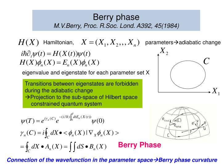
In the previous lesson, we introduced the Berry phase, a geometric phase acquired by a quantum state during a slow, cyclic evolution. We calculated it for the canonical example of a spin-1/2 particle in a precessing magnetic field and found that the phase is proportional to the solid angle traced by the magnetic field vector. This beautiful result connects quantum dynamics directly to geometry.

Today, we will generalize this powerful idea. Our goal is to derive the Berry connection and Berry curvature for a general two-band model. This is the essential theoretical step that allows us to apply the concept of geometric phase to the band structures of real materials. Instead of a magnetic field direction changing in time, our parameters will be the crystal momentum components, $k$ , as we move through the Brillouin zone. The resulting Berry curvature in momentum space is the key to understanding phenomena like the quantum Hall effect.

1. From Spin-1/2 to a General Two-Band Model

The spin-1/2 system you studied is more than just an example; it's the mathematical prototype for any two-level quantum system. A generic two-band model in condensed matter physics, which might arise from a tight-binding model with two orbitals per unit cell, can be described by a 2x2 Hamiltonian matrix, $H (k)$ .

Any 2x2 Hermitian matrix can be expressed as a linear combination of the identity matrix $σ_{0} = I$ and the three Pauli matrices $σ = (σ_{x}, σ_{y}, σ_{z})$ . Therefore, we can write our general two-band Hamiltonian as:

H (k) = d_{0} (k) I + d_{x} (k) σ_{x} + d_{y} (k) σ_{y} + d_{z} (k) σ_{z} = d_{0} (k) I + d (k) \cdot σ

Here, $d_{0} (k)$ and the components of the vector $d (k)$ are real functions determined by the specific physical system (e.g., hopping parameters, on-site energies).

This form is immediately familiar. It's mathematically identical to the Hamiltonian of a spin-1/2 particle in a magnetic field $B$ , where the vector $d (k)$ plays the role of the magnetic field.

The $d_{0} (k) I$ term simply shifts both energy levels by the same amount and has no effect on the eigenstates. Since the Berry phase depends only on the geometry of the eigenstates, we can ignore this term for our purposes.
The eigenvalues of $H (k)$ are then easily found: $E_{\pm} (k) = d_{0} (k) \pm ∣ d (k) ∣$ This gives us the dispersion relations for the upper (+) and lower (-) bands. An energy gap exists as long as $d (k) \neq = 0$ . Points in the Brillouin zone where $d (k) = 0$ correspond to band degeneracies, or band touching points.

The eigenstates, $∣ u_{\pm} (k)⟩$ , are the spinors pointing parallel (+) or anti-parallel (-) to the direction of the vector $d (k)$ . If we define a unit vector $d^(k) = d (k) /∣ d (k) ∣$ , then the problem of finding the geometric properties of the band structure is mapped exactly onto the problem of a spin in a "pseudo-magnetic field" $d (k)$ that varies with momentum $k$ .

Berry Phase and Curvature for a Spin-1/2 Particle — This image, which we saw in the context of a real magnetic field, is directly applicable here. Simply replace the parameter space `(Bx, By, Bz)` with `(dx, dy, dz)` and understand that this space is being explored by varying the crystal momentum **k**.

2. Berry Connection in Momentum Space

In the last lesson, we defined the Berry connection for a parameter $R$ as $A_{n} (R) = i ⟨ n (R) ∣ \nabla_{R} ∣ n (R)⟩$ . Now, our parameter is the momentum vector $k$ , and our eigenstates are the Bloch functions $∣ u_{n} (k)⟩$ . So, the Berry connection for the n-th band is:

A_{n} (k) = i ⟨ u_{n} (k) ∣ \nabla_{k} ∣ u_{n} (k)⟩

This vector field lives in momentum space and describes how the phase of the Bloch function twists as we move through the Brillouin zone.

As we discussed, the Berry connection is gauge-dependent. The choice of the overall phase of the eigenstates $∣ u_{n} (k)⟩$ at each $k$ can change $A_{n} (k)$ . This makes it an inconvenient quantity to work with directly. A much more useful, and physically observable, quantity is its curl: the Berry curvature.

3. Deriving the Berry Curvature

The Berry curvature is the momentum-space analogue of a magnetic field. In 3D, it's a vector defined as $Ω_{n} (k) = \nabla_{k} \times A_{n} (k)$ . In 2D, which is a common case, it has only one non-zero component, often written as $Ω_{n} (k) \equiv (Ω_{n})_{x y} = \partial_{k_{x}} (A_{n})_{y} - \partial_{k_{y}} (A_{n})_{x}$ .

Because the curvature is the curl of the connection, it is gauge-invariant, just as the magnetic field $B$ is invariant under gauge transformations of the vector potential $A$ .

To gain a deeper physical and mathematical understanding of the Berry connection and curvature, the following video provides an excellent summary of their properties and interrelations.

Deriving Berry phase, Berry connection & Berry curvature

The video 'Deriving Berry phase, Berry connection & Berry curvature' from Professor Nano offers a concise and clear explanation of the key concepts for this lesson.

Please watch the sections on the Berry connection and curvature (from 13:18 to 30:31). Pay special attention to: The definition of the Berry connection and its interpretation in terms of 'parallel transport' (Chapter 3). The discussion of gauge invariance, highlighting why the connection itself is not observable but the Berry phase over a closed loop is (Chapter 4). The definition of the Berry curvature as the curl of the connection and its direct analogy to the magnetic field (Chapter 5).

Now, let's derive a practical formula for the Berry curvature of our two-band model. While one could calculate the connection from the eigenstates and then take the curl, this is often cumbersome. A more direct and elegant formula exists.

For this derivation, we can consult an authoritative review article on the topic.

Berry phase effects on electronic properties

The review paper 'Berry phase effects on electronic properties' by Xiao, Chang, and Niu is a classic in the field. We will use it to find the definitive expression for the Berry curvature in a two-level system.

Please read section I.C.3, 'Example: The two-level system', focusing on equations (1.15) through (1.20). Observe how the authors map the generic two-level system to a spin Hamiltonian and then state the result for the Berry curvature.

The review paper provides the final result, which is both intuitive and powerful. For a Hamiltonian $H = d (k) \cdot σ$ , the Berry curvature vector for the two bands ( $\pm$ ) is given by:

Ω_{\pm} (k) = \pm \frac{1}{2} \frac{d}{∣ d ∣ ^{3}}

This expression, however, gives the curvature in the parameter space of $d$ . We need the curvature in our physical momentum space, $k$ . Using the chain rule for curls, one can derive a more useful expression. For a 2D system with momentum $k = (k_{x}, k_{y})$ , the single component of the Berry curvature is:

Ω_{x y}^{(\pm)} (k) = \pm \frac{1}{2∣ d ∣ ^{3}} d \cdot (\frac{\partial d}{\partial k _{x}} \times \frac{\partial d}{\partial k _{y}})

This can be simplified by using the unit vector $d^= d /∣ d ∣$ . The final, and most geometric, form is:

Ω_{x y}^{(\pm)} (k) = \pm \frac{1}{2} d^\cdot (\frac{\partial d ^}{\partial k _{x}} \times \frac{\partial d ^}{\partial k _{y}})

Let's unpack this important result:

The Berry curvature $Ω_{x y} (k)$ is a scalar field defined at each point in the 2D Brillouin zone.
It measures the "twisting" of the direction of the $d$ -vector as you move in momentum space.
The term $(\frac{\partial d ^}{\partial k _{x}} \times \frac{\partial d ^}{\partial k _{y}}) d k_{x} d k_{y}$ represents the vector area of the infinitesimal patch on the unit sphere of $d^$ directions, traced out as $k$ moves through an infinitesimal rectangle $d k_{x} d k_{y}$ .
Therefore, the Berry curvature $Ω_{x y} (k)$ is half the solid angle subtended per unit area of the Brillouin zone.
The curvature is non-zero only if the vector $d$ changes its direction as a function of $k$ . If $d (k)$ is always pointing in the same direction, the curvature is zero, and the band structure is topologically trivial.
The curvatures for the upper and lower bands are equal and opposite: $Ω_{x y}^{(+)} (k) = - Ω_{x y}^{(-)} (k)$ . This is a general property reflecting the fact that the total curvature summed over all bands is zero.

Berry Phase: Definition, Connection, and Curvature — This diagram summarizes the formalism. The Berry phase $\gamma_n(C)$ for a closed loop C in parameter space (our Brillouin zone) can be calculated either as a line integral of the Berry connection $A_n$ or, via Stokes' theorem, as a surface integral of the Berry curvature $B_n$ (which we denote $\Omega_n$).

Test your understanding!

Consider a simple 2D two-band model where $\mathbf{d}(\mathbf{k}) = (k_x, k_y, m)$, known as the massive Dirac model. What is the Berry curvature $\Omega_{xy}(\mathbf{k})$ for the lower band? Where is the curvature strongest?

Show answer

Let's calculate the necessary components for our formula: $Ω_{x y}^{(-)} (k) = - \frac{1}{2} d^\cdot (\frac{\partial d ^}{\partial k _{x}} \times \frac{\partial d ^}{\partial k _{y}})$ .

$d = (k_{x}, k_{y}, m)$
$∣ d ∣ = k_{x}^{2} + k_{y}^{2} + m^{2}$
$d^= \frac{1}{∣ d ∣} (k_{x}, k_{y}, m)$
$\frac{\partial d}{\partial k _{x}} = (1, 0, 0)$
$\frac{\partial d}{\partial k _{y}} = (0, 1, 0)$
$\frac{\partial d}{\partial k _{x}} \times \frac{\partial d}{\partial k _{y}} = (1, 0, 0) \times (0, 1, 0) = (0, 0, 1) = z^$

Now, plug these into the first formula for the curvature:

Ω_{x y}^{(-)} (k) = - \frac{1}{2∣ d ∣ ^{3}} d \cdot (\frac{\partial d}{\partial k _{x}} \times \frac{\partial d}{\partial k _{y}}) = - \frac{1}{2 ( k _{x}^{2} + k _{y}^{2} + m ^{2} ) ^{3/2}} (k_{x}, k_{y}, m) \cdot (0, 0, 1)

Ω_{x y}^{(-)} (k) = - \frac{m}{2 ( k _{x}^{2} + k _{y}^{2} + m ^{2} ) ^{3/2}}

This is a Lorentzian-like function centered at $k = 0$ . The curvature is strongest (most negative or positive, depending on the sign of $m$ ) at the origin $k = (0, 0)$ , where $∣ Ω_{x y} ∣ = \frac{1}{2∣ m ∣ ^{2}}$ . It decays rapidly as we move away from the origin. This concentration of Berry curvature near points of small band gaps (here, the gap at $k = 0$ is $2∣ m ∣$ ) is a very general and important feature.

Conclusion

In this lesson, we have successfully generalized the concepts of Berry phase from a specific spin model to any two-band system. This is the cornerstone for discussing topology in band structures.

Key Takeaways:

A general two-band Hamiltonian can be written as $H (k) = d_{0} (k) I + d (k) \cdot σ$ , mapping the problem to a spin in a $k$ -dependent pseudo-magnetic field $d (k)$ .
The Berry connection, $A_{n} (k) = i ⟨ u_{n} (k) ∣ \nabla_{k} ∣ u_{n} (k)⟩$ , is a vector potential in momentum space, but it is gauge-dependent.
The Berry curvature, $Ω_{n} (k) = \nabla_{k} \times A_{n} (k)$ , is a gauge-invariant "field" in momentum space that acts as a local measure of the topological character of the bands.
For a two-band model, the Berry curvature has a beautiful geometric interpretation: it is proportional to the solid angle subtended by the $d^$ vector per unit area of the Brillouin zone. The formula is $Ω_{x y}^{(\pm)} = \pm \frac{1}{2} d^\cdot (\partial_{k_{x}} d^\times \partial_{k_{y}} d^)$ .

Preview of the Next Lesson

We have now defined a local, gauge-invariant quantity—the Berry curvature—that lives in the Brillouin zone. What happens if we integrate this quantity over the entire Brillouin zone? Just as integrating the magnetic field flux over a closed surface gives a quantized charge (Gauss's law), integrating the Berry curvature over a closed momentum space (like the toroidal Brillouin zone) can yield a quantized integer. In the next lesson, we will define this integer, the Chern number, and see how it forms a topological invariant that classifies band structures.