Berry Phase for a Spin-1/2 in a Rotating Magnetic Field

Recommended resources

The freely available resources this lesson will direct you to.

Hello! Welcome to the next lesson in our course on condensed matter physics.

In our last lesson, we saw how the sign change of the $d$ -wave superconducting order parameter—a property of its phase—leads to profound and measurable physical consequences. This idea that the phase of a quantum wavefunction can carry deep physical information beyond the simple time evolution is a central theme in modern physics. Today, we will explore this concept in its most general and fundamental form by introducing the Berry phase.

Our goal in this lesson is to define the Berry phase and calculate it for a canonical example: a spin-1/2 particle in a slowly rotating magnetic field. This will lay the groundwork for understanding how geometry and topology manifest in quantum mechanics, which is the key to unlocking the physics of topological materials.

We will begin by developing the concept of the Berry phase from the adiabatic theorem. Then, we will perform the explicit calculation for the spin-1/2 system and see how a purely geometric quantity—a solid angle—emerges from the quantum dynamics.

1. The Adiabatic Theorem and the Birth of a Geometric Phase

Let's consider a quantum system described by a Hamiltonian $H (R (t))$ that depends on a set of parameters $R$ which are varied slowly in time. The adiabatic theorem states that if the system starts in the $n$ -th eigenstate of the initial Hamiltonian, $∣ n (R (0))⟩$ , it will remain in the instantaneous $n$ -th eigenstate, $∣ n (R (t))⟩$ , throughout the evolution, provided the change is slow enough.

The evolution of the wavefunction acquires a phase. You are already familiar with the dynamical phase, $θ_{n} (t)$ , which depends on the energy of the state:

θ_{n} (t) = - \frac{1}{ℏ} \int_{0}^{t} E_{n} (R (t^{'})) d t^{'}

In 1984, Sir Michael Berry showed that there is an additional phase, $γ_{n} (t)$ , which depends not on how long the evolution takes, but on the path the system traces in its parameter space. This is the geometric phase, or Berry phase.

To get a conceptual feel for this, please watch the beginning of the following video.

Deriving Berry phase, Berry connection & Berry curvature

This video from the channel Professor Nano provides an excellent conceptual introduction to the Berry phase. It explains its origin in adiabatic evolution and introduces the beautiful analogy of parallel transport on a curved surface.

Please watch the first 3 minutes of the video (00:00 - 03:09). Focus on the distinction between an open path and a closed loop, and the idea that the phase depends on the 'twist' of the eigenstates in parameter space.

The key idea is that as the Hamiltonian changes, the eigenstates themselves 'rotate' in Hilbert space. The Berry phase quantifies the accumulated phase from this rotation.

2. Formal Derivation and Gauge Invariance

Let's now formalize this. Given the adiabatic theorem, we write the full time-evolved state as:

∣ Ψ_{n} (t)⟩ = e^{i γ_{n} (t)} e^{i θ_{n} (t)} ∣ n (R (t))⟩

Substituting this into the time-dependent Schrödinger equation, $i ℏ \frac{\partial}{\partial t} ∣ Ψ_{n} (t)⟩ = H (R (t)) ∣ Ψ_{n} (t)⟩$ , and solving for the Berry phase $γ_{n} (t)$ yields a crucial result.

The following video provides a clear, step-by-step derivation. Your background in quantum mechanics should make the formalism very familiar.

Deriving Berry phase, Berry connection & Berry curvature

This segment of the same video derives the expression for the Berry phase from the Schrödinger equation. It's a standard and elegant derivation that clearly separates the geometric phase from the dynamical part.

Watch from 03:09 to 10:03. Follow the substitution of the state ansatz into the Schrödinger equation. Pay close attention to how the time derivative of the Berry phase, \dot{\gamma}_n, is isolated and how the final expression is transformed from a time integral to a line integral in parameter space.

As the video shows, the time derivative of the Berry phase is:

γ ˙_{n} (t) = i ⟨ n (R (t)) ∣ \frac{d}{d t} ∣ n (R (t))⟩

Using the chain rule, $\frac{d}{d t} = R ˙ \cdot \nabla_{R}$ , we can rewrite the total Berry phase accumulated over a path $C$ in parameter space (from $t = 0$ to $t = T$ ) as a line integral:

γ_{n} (C) = \int_{0}^{T} γ ˙_{n} (t) d t = \int_{C} i ⟨ n (R) ∣ \nabla_{R} ∣ n (R)⟩ \cdot d R

This is the central result. The phase $γ_{n} (C)$ depends only on the path $C$ in parameter space, not on how quickly it is traversed.

Berry Connection and Gauge Invariance

The vector field inside the integral is of fundamental importance. We define the Berry connection (or Berry vector potential) as:

A_{n} (R) = i ⟨ n (R) ∣ \nabla_{R} ∣ n (R)⟩

So the Berry phase is simply $γ_{n} (C) = \int_{C} A_{n} (R) \cdot d R$ . This is formally analogous to the expression for the magnetic flux in electromagnetism being the integral of the vector potential.

However, there's a subtlety. In quantum mechanics, the phase of an eigenstate is arbitrary. We can redefine our instantaneous eigenstates by a local phase factor:

∣ n^{'} (R)⟩ = e^{i χ (R)} ∣ n (R)⟩

This is a gauge transformation. How does this affect our physical quantity, the Berry phase? Under this transformation, the Berry connection changes as:

A_{n}^{'} (R) = A_{n} (R) - \nabla_{R} χ (R)

This is exactly how the magnetic vector potential transforms in E&M! Because $A_{n}$ is gauge-dependent, it is not by itself a physical observable.

What about the Berry phase, $γ_{n} (C)$ ? If the path $C$ is an open path from $R_{i}$ to $R_{f}$ , the phase changes by $χ (R_{i}) - χ (R_{f})$ , so it is not gauge-invariant.

However, if the path is a closed loop ( $R (T) = R (0)$ ), the situation changes dramatically. The change in the Berry phase is:

Δ γ_{n} (C) = - \oint_{C} \nabla_{R} χ (R) \cdot d R = χ (R (0)) - χ (R (T)) = 0

The total Berry phase $γ_{n} (C)$ for a closed loop is gauge-invariant (up to integer multiples of $2 π$ ). This means it is a physically observable quantity.

3. Example: Spin-1/2 in a Rotating Magnetic Field

The abstract formalism becomes clear with a concrete example. Let's calculate the Berry phase for a spin-1/2 particle (like an electron) whose spin is coupled to an external magnetic field $B$ that is slowly precessing around a cone.

The Hamiltonian is:

H (t) = - μ \cdot B (t) = \frac{μ _{B} g}{ℏ} S \cdot B (t)

We'll assume the magnetic field $B (t)$ traces a circle at a fixed polar angle $θ$ with a constant angular velocity $ω$ . The parameter space here is the direction of $B$ , which can be parameterized by the spherical coordinates $(θ, ϕ)$ . The path is a closed loop where $ϕ$ goes from 0 to $2 π$ .

The following resource provides a concise derivation of the Berry phase for this exact problem.

Review of Berry phase

These notes by Ming-Che Chang provide a very clear and self-contained calculation for the spin-1/2 example. This will be our guide for the calculation.

Please read the section titled 'Example' (from Eq. 1.17 to Eq. 1.24). Focus on understanding the setup: the Hamiltonian, the eigenstates, and the goal of calculating the Berry phase for a closed loop at constant heta.

Let's break down the calculation.

1. The Eigenstates:
The Hamiltonian can be written as $H = μ_{B} B (σ \cdot n^)$ , where $n^$ is the unit vector along $B$ . The eigenstates are the spin-up and spin-down states along the instantaneous direction $n^= (sin θ cos ϕ, sin θ sin ϕ, cos θ)$ . As given in the notes, for the spin-up state (energy $+ μ_{B} B$ ), the eigenstate is:

∣ n^, + ⟩ = (cos (θ /2) e^{i ϕ} sin (θ /2))

2. The Berry Connection:
Our parameter space is the surface of a sphere, described by $(θ, ϕ)$ . The gradient operator in spherical coordinates is $\nabla = r^\frac{\partial}{\partial r} + θ^\frac{1}{r} \frac{\partial}{\partial θ} + ϕ^\frac{1}{r s i n θ} \frac{\partial}{\partial ϕ}$ . For our purposes, we are interested in the direction of the field, so we can set $r = B$ and focus on the angular components. The Berry connection $A_{+} (B) = i ⟨ n^, + ∣ \nabla_{B} ∣ n^, + ⟩$ can be calculated.

Let's compute the $ϕ$ -component, which is what we'll need for our integral around a loop of constant $θ$ :

(A_{+})_{ϕ} = i ⟨ n^, + ∣ \frac{1}{B sin θ} \frac{\partial}{\partial ϕ} ∣ n^, + ⟩

The derivative acts only on the $e^{i ϕ}$ term in the eigenstate:

\frac{\partial}{\partial ϕ} ∣ n^, + ⟩ = (0 i e^{i ϕ} sin (θ /2))

Taking the inner product:

⟨ n^, + ∣ \frac{\partial}{\partial ϕ} ∣ n^, + ⟩ = (cos (θ /2), e^{- i ϕ} sin (θ /2)) (0 i e^{i ϕ} sin (θ /2)) = i sin^{2} (θ /2)

Plugging this back into the expression for $(A_{+})_{ϕ}$ gives:

(A_{+})_{ϕ} = i (\frac{1}{B sin θ}) (i sin^{2} (θ /2)) = - \frac{sin ^{2} ( θ /2 )}{B sin θ} = - \frac{1 - cos θ}{2 B sin θ}

The full Berry connection vector is $A_{+} = (A_{+})_{ϕ} ϕ^$ .

3. The Berry Phase:
Now we integrate along our closed loop $C$ , which is a path of constant $θ$ where $ϕ$ goes from 0 to $2 π$ . The line element is $d l = (B sin θ) d ϕ ϕ^$ .

γ_{+} (C) = \oint_{C} A_{+} \cdot d l = \int_{0}^{2 π} (A_{+})_{ϕ} (B sin θ) d ϕ

γ_{+} (C) = \int_{0}^{2 π} (- \frac{1 - cos θ}{2 B sin θ}) (B sin θ) d ϕ = - \frac{1 - cos θ}{2} \int_{0}^{2 π} d ϕ = - π (1 - cos θ)

This is a remarkable result! The phase acquired has nothing to do with the magnitude of the field $B$ or how fast it precesses ( $ω$ ). It depends only on the geometry of the path—specifically, the polar angle $θ$ .

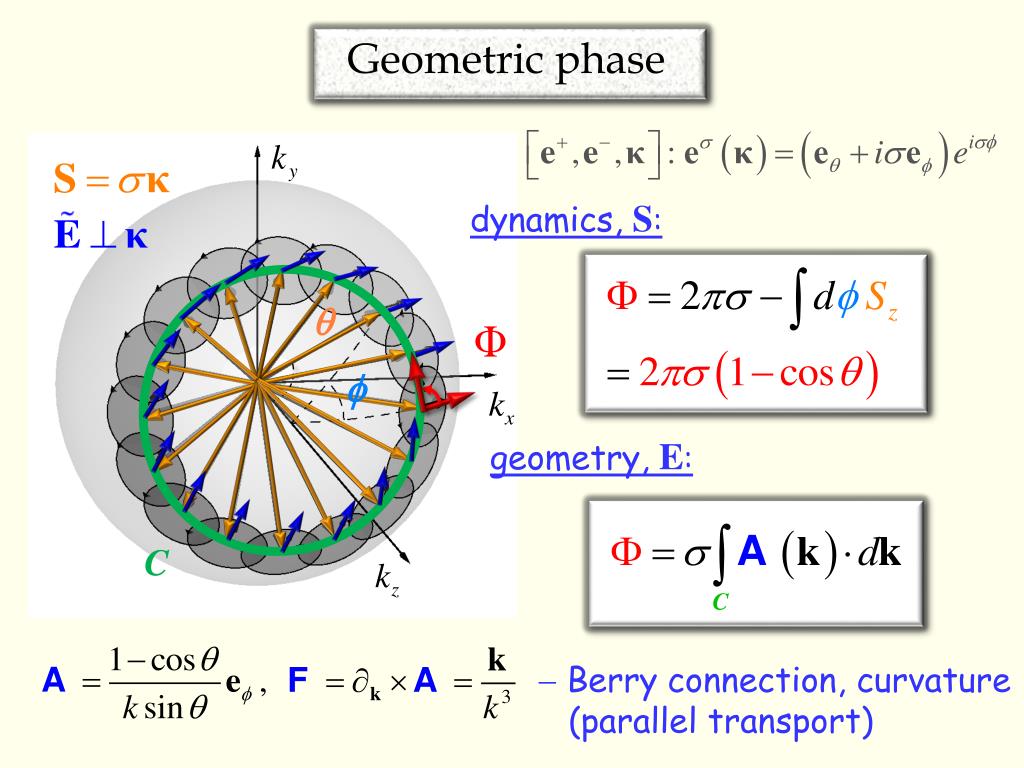
The quantity $2 π (1 - cos θ)$ is the solid angle $Ω (C)$ subtended by the circular path on the sphere as viewed from the origin. So, we find:

γ_{+} (C) = - \frac{1}{2} Ω (C)

The geometric phase is half the solid angle traced by the path in parameter space. For the spin-down state, the calculation yields $γ_{-} (C) = + \frac{1}{2} Ω (C)$ . This intimate connection between a quantum phase and a classical geometric quantity is the essence of Berry's discovery.

Geometric Phase and Berry Phase for a Spin-1/2 Particle — A visual summary of the spin-1/2 case. The vector $\mathbf{S}$ (or $\mathbf{B}$) precesses, tracing a path on a sphere. The Berry phase $\Phi_G$ is directly proportional to the solid angle $\Omega$ enclosed by this path. The Berry connection $\mathbf{A}$ and curvature $\mathbf{F}$ are the mathematical tools used to formalize this relationship.

Test your understanding!

The notes in resource LINK also give an expression for the Berry curvature, $F_{\pm} (B) = \nabla_{B} \times A_{\pm} (B)$ . For the spin-up case, this is $F_{+} (B) = - \frac{1}{2} \frac{B ^}{B ^{2}}$ . This looks like the magnetic field of a magnetic monopole at the origin!

Using this fact and Stokes' theorem, $γ (C) = \oint_{C} A \cdot d l = \iint_{S} (\nabla \times A) \cdot d S$ , can you re-derive the Berry phase $γ_{+} (C)$ by integrating the Berry curvature over the spherical cap surface $S$ enclosed by the loop $C$ ?

Show answer

We need to calculate the surface integral $\iint_{S} F_{+} \cdot d S$ .
The surface element on a sphere of radius $B$ is $d S = B^{2} sin θ^{'} d θ^{'} d ϕ^{'} B^$ .
The integral becomes:

γ_{+} (C) = \iint_{S} (- \frac{1}{2} \frac{B ^}{B ^{2}}) \cdot (B^{2} sin θ^{'} d θ^{'} d ϕ^{'} B^)

γ_{+} (C) = - \frac{1}{2} \int_{0}^{2 π} d ϕ^{'} \int_{0}^{θ} sin θ^{'} d θ^{'}

The integral over $ϕ^{'}$ gives $2 π$ . The integral over $θ^{'}$ gives $[- cos θ^{'}]_{0}^{θ} = 1 - cos θ$ .
Putting it all together:

γ_{+} (C) = - \frac{1}{2} (2 π) (1 - cos θ) = - π (1 - cos θ)

This confirms our result from the line integral. The Berry phase can be viewed as the "flux" of the Berry curvature through the loop.

Conclusion

In this lesson, we have formally introduced the Berry phase, a geometric phase acquired by a quantum state during an adiabatic cyclic evolution.

Key Takeaways:

The total phase acquired by an adiabatically evolving state has a dynamical part (dependent on energy and time) and a geometric part (dependent on the path in parameter space).
The geometric phase, or Berry phase, is calculated by the line integral of the Berry connection $A_{n}$ around a closed path in the system's parameter space.
The Berry phase is gauge-invariant for closed loops, making it a physically observable quantity.
For a spin-1/2 particle in a precessing magnetic field, the Berry phase is directly proportional to the solid angle traced by the magnetic field vector, explicitly revealing its geometric nature.

Preview of the Next Lesson

We have defined the Berry phase and its associated Berry connection, $A$ , and calculated them for a specific, important example. We also briefly encountered the Berry curvature, $F = \nabla \times A$ , which acts like a "magnetic field" in parameter space. In our next lesson, we will elevate these concepts from a specific example to a general framework. We will derive the Berry connection and Berry curvature for a general two-band model, which is the essential theoretical tool needed to understand the topological properties of materials like Chern insulators and the quantum Hall effect.