Recommended resources
The freely available resources this lesson will direct you to.
Hello. The previous lesson examined how coatings, aspheres, and moving groups expanded what designers could build. The remaining question is how to judge the resulting lens. A claim that it “resolves” fine lines says little about whether it preserves contrast across the frame, illuminates the corners, handles bright lights, or places image detail where it belongs.
In this final lesson on optical image engineering, you will build a multidimensional lens evaluation. We will connect modulation transfer, vignetting, flare, distortion, and telecentricity to different physical failures—and to the photographic tasks for which those failures matter. Allow about 40–45 minutes, including the selected viewing and reading.
Contrast transfer: more informative than a resolution limit
Imagine imaging a sinusoidal pattern whose brightness varies between and . Its modulation is
At a specified spatial frequency, the modulation transfer function (MTF) is the image modulation divided by the object modulation, after accounting for magnification when relating object and image spatial frequencies. Frequency is commonly reported in line pairs—or cycles—per millimetre at the image plane. An MTF of 0.7 means the image retains 70% of the input pattern’s modulation under the stated test conditions. By convention, MTF is normalized to one at zero frequency.
This answers a question that a limiting-resolution figure cannot: how much contrast survives at the scales you need? Two lenses might both distinguish a very fine test pattern, yet one could render moderately fine textures with much stronger contrast. MTF must therefore be read at relevant frequencies, not reduced to the last frequency at which lines remain discernible.
Watch the introduction and graph-reading portions of Ansys Learning’s Modulation Transfer Function (MTF) — Lesson 5. The later aperture comparison is a useful reminder that a better diffraction limit need not mean better actual performance.
Modulation Transfer Function (MTF) — Lesson 5
Ansys Learning’s video introduces contrast transfer and identifies the axes and line styles on an MTF plot. Watch it as a guide to reading plots, rather than as a complete model of a photographic lens.
Watch MTF and curves for the definition, spatial-frequency axis, diffraction reference, and sagittal and tangential traces. Then watch aperture comparison: distinguish the diffraction-limited reference from the aberration-affected lens curves.
For a standards-oriented account, read the definition and measurement priorities in the independent broadcast-lens guideline Technical Guidelines from ARD. Its numerical requirements concern particular HD applications, not all photographic formats.
[PDF] Technical Guidelines - ARD
Read ARD’s treatment of MTF to see which measurement conditions a practical lens specification must make explicit.
On printed p. 8, in Section 3.1, “Sharpness and Resolution,” start at “Definition: The modulation transfer factor.” Read the definition and the immediately following requirements for frequency, image field, focal length, and colour. Continue from “The following parameters shall be documented” through the measurement list; notice the separate attention given to off-axis positions and radial versus tangential measurements. Stop before “Parameter range.”
The MTF plot below holds aperture and working distance fixed while changing field height and pattern orientation. Its black curve is a diffraction-limited reference for the plotted conditions; the coloured curves represent lens performance. The gap between them is a way to see what the real optical design loses beyond that reference.
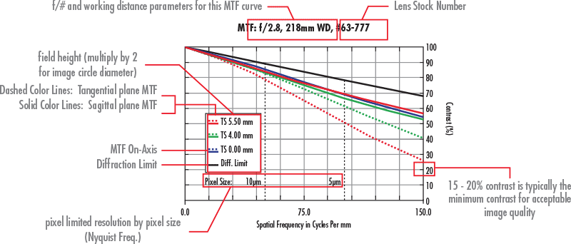
Read such a plot in three directions. Moving right asks about progressively finer detail. Moving from centre to edge asks whether that detail survives across the image circle. Comparing sagittal and tangential curves asks whether performance depends on pattern orientation. A separation between those orientations is evidence of anisotropic off-axis imaging; astigmatism is one possible contributor, but an MTF plot alone does not uniquely diagnose its cause. Wavelength, focus setting, field curvature, and manufacturing alignment can also change the curves.
The appropriate frequency range depends on the recording system and output. For a sensor with pixel pitch , the one-dimensional sampling Nyquist frequency is : approximately 50 cycles/mm for pixels and 100 cycles/mm for pixels. Nyquist is not a guarantee that all detail below it will be faithfully captured. Pixel aperture reduces contrast, while frequencies above Nyquist can alias. Under suitable linear, shift-invariant assumptions, optical and sensor transfer functions can be combined to predict system response; multiplying supposed “MTFs of individual lens elements” is not, in general, a valid shortcut. Nor does MTF describe every property of a lens: the next four metrics address information it leaves out.
Field illumination: where the photons go
A uniformly bright scene need not produce a uniformly illuminated image. Define relative field illuminance at image height as , the irradiance relative to the centre under a specified test setup. If the corner value is 0.75, it receives three-quarters of the centre irradiance—about 0.42 exposure stops less.
Two effects must be distinguished. Mechanical or optical vignetting occurs when an oblique ray bundle has part of its pupil obstructed by a mount, element, or other aperture. It can be particularly strong wide open and often diminishes on stopping down. Natural illumination fall-off occurs even without that obstruction because the geometry of oblique imaging changes the flux delivered per image area. The familiar law describes an important idealized configuration; pupil geometry and lens design determine how closely a real lens follows it. Stopping down need not remove this natural component.
Read the illumination definition and dependencies in the ARD guideline, together with its short definitions of geometric distortion and veiling glare. These give three quantities that a sharpness chart cannot supply.
[PDF] Technical Guidelines - ARD
Use these short sections of ARD’s guideline to connect each defect to a separately measured quantity. Treat its numerical limits as specifications for its stated broadcast applications.
On printed pp. 13–14, in Section 3.4, “Relative Field Illuminance,” start at “Definition: The relative field illuminance.” Read the definition and requirement, ending after the corner-illumination figure. On printed pp. 15–16, in Section 3.6, “Picture height distorsion,” read from “Definition: The picture height distortion” through the distortion limit. Finally, on printed pp. 16–17, in Section 3.8, “Flare, Veiling glare,” read from “Definition: The veiling glare index” through the glare criterion.
Relative illumination matters beyond whether corners look dark. Brightening a vignetted digital image afterward also amplifies its corner noise; if exposure was set to protect highlights at the centre, the darker corners received fewer photons. A lens with excellent corner MTF but severe fall-off can thus deliver sharp yet noisy corner detail. Conversely, a moderate amount of fall-off may be acceptable for a centred subject. Evaluate illumination at the apertures, focal lengths, focus distances, and format you intend to use.
Flare and distortion: two ways a sharp image can be wrong
Last lesson distinguished ghosts from veiling flare. Here is why veiling flare evades an ordinary MTF comparison. Suppose a bright surrounding scene adds approximately uniform stray-light irradiance to a dark-and-bright test pattern. Its observed modulation becomes
The unwanted light raises both measured intensities, leaving their difference unchanged but reducing their ratio. In an actual photograph, depends on the brightness and placement of sources, including sources just outside the frame. A conventional MTF measurement in controlled lighting may therefore miss the contrast loss a lens exhibits when photographing a backlit subject. Ghosts are different again: they add structured, displaced light, not merely a uniform veil.
A useful flare assessment records the position and intensity of a bright source, the aperture, and whether the artifact is a broad veil or a distinct ghost. Test near-frame as well as in-frame sources. The ARD guideline’s veiling glare index—light measured in an image of a black area relative to its bright surround—makes this a measurable contrast problem. Its cited 2% criterion is a requirement under a specified test method, not a universal visibility threshold for every scene.
Distortion, by contrast, is a position error. For an otherwise rectilinear image, a simple radial model is
Negative radial displacement toward the axis gives barrel distortion; positive displacement gives pincushion distortion. Straight lines away from the image centre can consequently bow outward or inward. A lens can have high local MTF and still put those crisp lines in the wrong places. Distortion should also not be confused with the perspective effects of changing camera position.
A grid test assesses position rather than sharpness. Align camera and grid carefully: tilt can introduce converging lines that are not lens distortion. Software can remap a distorted image, but that may require cropping and interpolation, so correction is not always free. For architectural recording or measurement, small geometric error may be decisive; for another photographic use, stronger distortion might be tolerable.
Telecentricity: the angle at which the image arrives
The chief ray of a field-point bundle passes through the centre of the aperture stop. In an image-space telecentric lens, chief rays arrive nearly parallel to the optical axis across the image field. Equivalently, the exit pupil—the apparent image of the stop as seen from image space—is very far from the image plane. If its effective distance is , a simple geometric estimate for chief-ray angle at image height is . Moving the apparent pupil farther away reduces the variation of that angle across the frame.

This is not the same as making the converging ray cone narrow. F-number governs its aperture angle; telecentricity concerns the direction of the cone’s centre as field position changes. Even a strongly image-space telecentric fast lens sends rays through a range of angles around each chief ray.
Read the explanation of exit-pupil position and beam tilt in H. H. Nasse’s Distagon, Biogon, Hologon, published by Zeiss. It provides a particularly useful engineering comparison between wide-angle designs. Its examples are concrete designs, not rules that every lens bearing a design-family name must obey.
Read Nasse’s comparison to see how excellent image geometry, field illumination, and compatibility with a sensor can pull a wide-angle design in different directions.
On printed p. 12/15, start in the paragraph beginning “The exit pupil is the area.” Read the pupil comparison, including the numbered discussion of natural and artificial fall-off. Continue through the sensor comparison; note why chief-ray angle has become an interface constraint. For the geometry trade-off, turn to printed p. 10/15 and read the paragraph beginning “In addition to excellent contrast” through the distortion comparison.
Large chief-ray angles can reduce the efficiency or uniformity with which a pixel’s microlens and light-sensitive region collect light, and can complicate performance through glass placed in front of the sensor. Film and sensors therefore place different constraints on the same optical layout. More telecentricity can help, but it may demand larger rear optics and mount clearances. The historical move from film to electronic capture did not merely replace the recording material; it changed what counts as a well-matched lens–recording-plane system.
Making a defensible lens choice
A useful evaluation begins with a use case, then specifies tests at matching conditions. Compare lenses at the same image format, relevant aperture and focus distance, equivalent field positions, and appropriate wavelengths or colour channels. For a zoom, repeat at representative focal lengths. Record whether a result comes from an optical-bench lens measurement or from a complete camera: sensor sampling, processing, and sharpening can affect the latter.
The following hypothetical comparison shows why “the sharper lens” is not always a meaningful verdict. Assume both are tested at the same f-number and format; MTF entries are at the same image-plane frequency.
| Measurement | Lens A | Lens B |
|---|---|---|
| Centre / corner MTF | 0.88 / 0.32 | 0.80 / 0.65 |
| Corner relative illuminance | 0.48 | 0.78 |
| Maximum barrel distortion | 3% | 0.5% |
| Veiling glare index under one common test | 4% | 1% |
| Corner chief-ray angle |
Lens A wins on central contrast transfer at that frequency. Lens B is the stronger candidate for uniformly detailed, geometrically faithful images on a sensor sensitive to oblique rays: its corners retain more contrast and light, its distortion is smaller, and its chief rays arrive less obliquely. But this table cannot settle cost, size, focal length, other spatial frequencies, close-focus behaviour, or how either lens reacts to a particular bright source. It is a decision framework, not a universal ranking.
That is the central discipline of lens evaluation: ask which information must survive, where in the frame, and under what illumination and recording conditions. MTF addresses contrast by scale and location; field illuminance addresses photon distribution; flare addresses stray light; distortion addresses position; and telecentricity addresses the angular interface with the recording plane.
Conclusion
A single resolution number discards most of what makes a photographic lens usable. Read MTF across frequency, field, and orientation, but pair it with illumination, stray-light, geometry, and chief-ray measurements under specified conditions. Those metrics can disagree without any test being wrong: they measure different physical properties.
This completes the optical-image module. Next, the course turns from forming an image to making it permanent, beginning with how absorbed photons create a developable latent image in silver-halide material.