Image Distance, Magnification, and Field of View in Pinhole and Thin-Lens Cameras

Hello. This course follows the camera as an engineering system: first the optics that form an image, then the materials that record it, the mechanisms that control exposure and focus, and finally electronic sensors and computational imaging. We begin with the geometric model behind both the camera obscura and the photographic lens.

In this lesson, you will derive where an image forms, how large it is, and how much of a scene fits on the recording surface. The distinction to watch is simple but consequential: a pinhole projects onto a plane you choose; a lens focuses an object plane onto a plane determined by its focal length.

A pinhole: projection without focusing

Imagine an object in front of a tiny hole, with a recording surface behind it. In the ideal geometric model, only one ray from each object point passes through the hole. Where that ray meets the surface is the point’s image location.

The diagram below shows both the physical sensor, to the left of the camera center, and a virtual image plane, to its right. The latter is a convenient way to draw upright projection coordinates; it is not a second sensor.

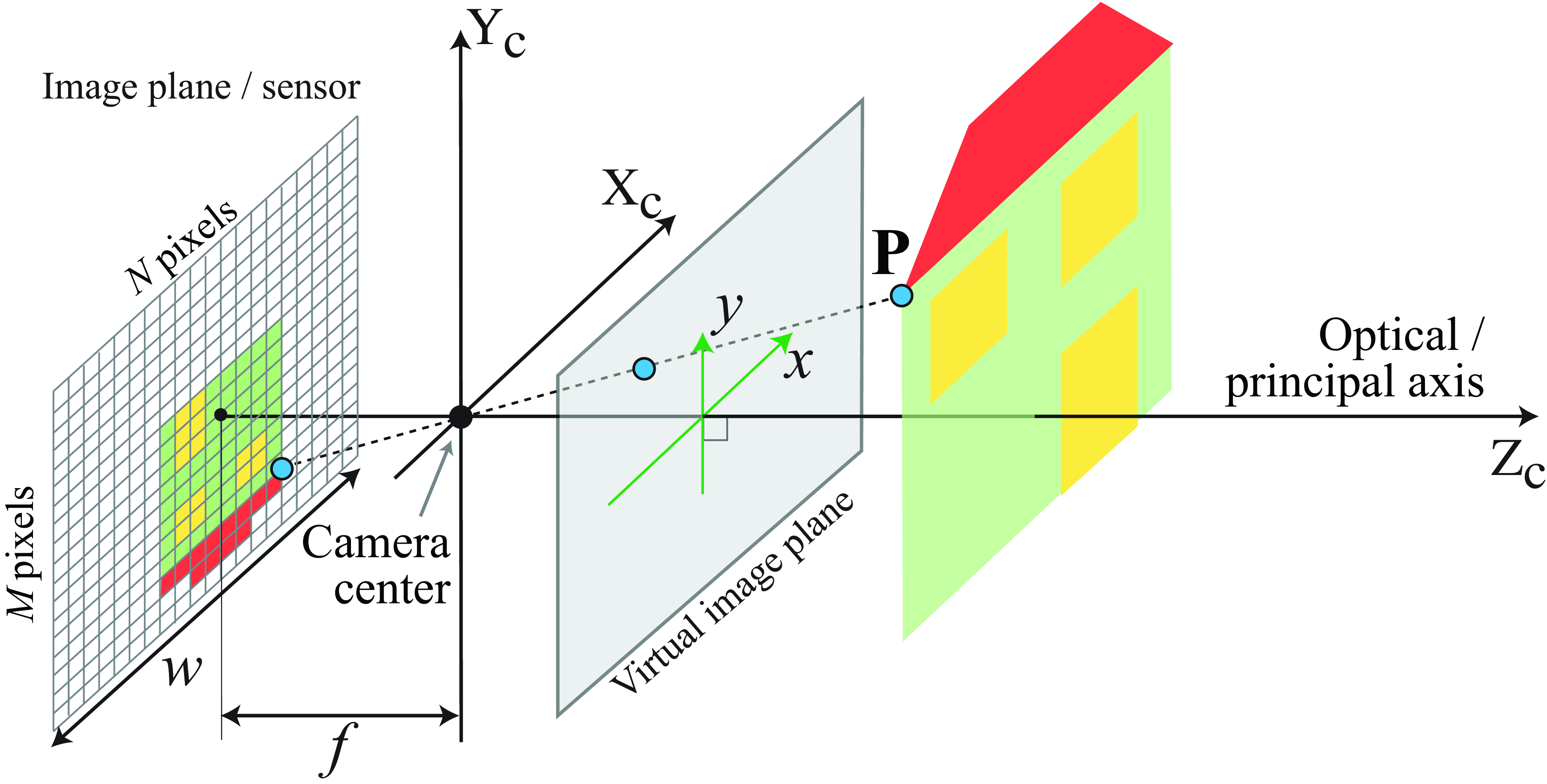
Set the hole at the origin and point the $Z$-axis toward the scene. An object point has coordinates $(X,Y,Z)$, where $Z>0$. Put the physical sensor at $Z=-d$, with $d>0$. The ray through the origin has transverse coordinates proportional to its axial coordinate, so similar triangles give

The minus signs express inversion. If instead we draw a virtual plane at $Z=+d$, its coordinates are $x_{\mathrm{v}}=dX/Z$ and $y_{\mathrm{v}}=dY/Z$. Keeping these two planes distinct prevents a common sign error when moving between photographic diagrams and computer-vision projection equations.

Watch the following explanation for the ray geometry and for why projected scale depends on object depth. Its presentation uses a virtual image plane; translate its coordinates to the physical sensor using the minus signs above.

Suppose a flat object of height $H$ lies perpendicular to the optical axis at depth $Z=u$. Apply the projection equation to its top and bottom: their separation on the physical sensor is $-dH/u$, if upward object height and sensor height use the same coordinate direction. The signed transverse magnification is therefore

This is a scale for an object at a specified depth, not a single scale for an entire three-dimensional scene. Two equally tall objects at different depths have different image heights.

Notice what this derivation does not specify: a required sensor distance. In an ideal pinhole camera, you can move the sensor to another distance $d$ and still intercept one projected ray per object point. Image size changes, but there is no thin-lens focusing equation. A real hole has finite diameter, so “one ray” is an idealization; we will examine the resulting resolution trade-offs later in this module.

A thin lens: making many rays meet

A pinhole rejects nearly all the rays arriving from an object point. A lens offers a different solution: admit rays across an aperture and refract them so that they meet again at an image point. Its shape and refractive index determine its focal length $f$. Here, paraxial means that ray heights and angles are small enough for the small-angle approximation to describe their paths; thin lens means that we neglect the separation between the lens’s refracting surfaces when tracing the rays.

The optical origin of this model is worth seeing before using it. In Section 6.2, “Lensmaker’s Formula,” of Foundations of Computer Vision, follow how small-angle Snell refraction connects surface curvature to focal length. You need not memorize the particular symmetric-lens curvature formula; the important result here is that, within this approximation, the lens supplies a definite focusing power.

Now put a converging thin lens at the origin. An upright object of height $H$ is at distance $u>0$ in front of it. If a real image forms, let its plane be at distance $v>0$ behind the lens, with signed image height $h_{\mathrm{i}}<0$. Trace two rays from the object’s top:

1. The central ray passes through the ideal thin lens’s center without changing direction. Similar triangles give $h_{\mathrm{i}}/H=-v/u$.
2. A ray parallel to the optical axis reaches the lens at height $H$, then passes through the rear focal point at distance $f$. At the image plane, its height is $H(1-v/f)$.

Both rays must reach the same image point. Equating their heights and cancelling $H$ gives

Solving for the image distance, then returning to the central ray, yields

This derivation assumes $u>f$, so that $v>0$ and a real image can be placed on a sensor. An object at $u=f$ sends the ideal outgoing rays parallel, giving no finite real-image distance; an object inside $f$ does not form a real image behind this lens.

There is also a compact way to read the equation in terms of ray slopes. For an axial object point, a ray reaching lens height $h$ has incoming paraxial slope $h/u$, measured along its direction of travel. To reach the axial image point, its outgoing slope must be $-h/v$. The lens changes that slope by $-h/f$. Thus $-h/v-h/u=-h/f$: the reciprocal-distance equation is a statement of how much convergence the lens must add.

Section 6.3, “Imaging with Lenses,” in Foundations of Computer Vision gives the corresponding central-ray and focal-ray rules. One caution: its numbered rule 4 states the magnification ratio as $a/b$. With its definitions of $a$ as object distance and $b$ as image distance, the image-to-object height ratio instead has magnitude $b/a$, as the central-ray triangles above show.

The limiting cases make the equations easier to interpret. As $u$ becomes very large, $1/u$ becomes negligible and $v$ approaches $f$: a lens focused on a distant scene places its sensor approximately one focal length behind the lens. At $u=2f$, the image also lies at $2f$ and has the same size as the object, inverted. Moving the object closer to $f$ pushes the required image plane farther away and increases $|m|$. A fixed sensor plane cannot therefore sharply image every object distance at once.

Field of view: which directions reach the frame?

Field of view is an angular extent, so it needs both a direction—horizontal, vertical, or diagonal—and a definition of the frame size. Let the sensor width be $W$. For the ideal pinhole, a ray from a scene direction at half-angle $\alpha$ to the optical axis meets the sensor edge at transverse distance $W/2$. The right triangle at the hole gives

For the ideal thin lens focused at object distance $u$, replace the pinhole-to-sensor distance by the image distance $v$:

At distant focus, $v\approx f$, giving the familiar photographic expression

Use sensor height in place of $W$ for vertical field of view, or the sensor diagonal for diagonal field of view. The arctangent follows from the right-triangle geometry; treating the lens as a thin, well-behaved imaging system is the approximation. A real wide-angle lens need not obey this ideal rectilinear model all the way to its frame edge.

The geometrical-optics notes Section 3 Imaging With A Thin Lens provide a useful diagrammatic check. Their “Field of View” slides distinguish half-angle from full angle and show why a rectangular detector has different horizontal, vertical, and diagonal fields.

Consider a $50\mathrm{mm}$ thin lens and a $36\mathrm{mm}$-wide sensor. Focused at infinity, its horizontal field of view is $2\arctan (36/100)$, approximately $39.6^{\circ }$. If an object is $1000\mathrm{mm}$ from the lens, however, the image equation gives $v\approx 52.6\mathrm{mm}$. The horizontal angular field for that focused object plane is then about $37.8^{\circ }$, and a $200\mathrm{mm}$-tall object in that plane produces an inverted image about $10.5\mathrm{mm}$ tall. Using $f$ in place of $v$ is excellent for distant scenes, but this example shows precisely where the approximation enters.

Equivalently, the object-plane width captured at distance $u$ is $uW/v$: magnification tells you how much object fits across the sensor, while field of view expresses the same geometry as an angle at the camera.

What to retain

A pinhole maps scene points by similar triangles; its sensor spacing $d$ sets image scale and angular coverage, but is not a focusing distance. A thin lens uses refraction to bring many rays from a point together. For a real image of an object beyond its focal length, its image distance and signed magnification are

Finally, for sensor width $W$, the ideal horizontal field of view is $2\arctan [W/(2v)]$, with $v\approx f$ at distant focus. These relationships are the geometric baseline for the rest of the optics module. Next, we will ask what they leave out: how much light the lens admits, and how aperture size determines image-plane irradiance and throughput.