BFS and DFS: Algorithms and Applications

Hello! Welcome to your next lesson in the Graph Algorithms and Applications module.

In our previous lesson, we focused on the crucial first step of modeling real-world problems as graphs. You learned how to represent task dependencies as Directed Acyclic Graphs (DAGs), resource conflicts using graph coloring, and potential deadlocks with resource allocation graphs.

Now that we can represent problems using graphs, our next step is to learn how to navigate them. This lesson introduces the two fundamental algorithms for graph traversal: Breadth-First Search (BFS) and Depth-First Search (DFS). These algorithms are the building blocks for many more complex graph operations and are a staple of technical interviews.

Our learning outcome for today is to implement Breadth-First Search (BFS) and Depth-First Search (DFS) and explain their distinct use cases. We will implement them in Python and, more importantly, develop a strong intuition for when to choose one over the other.

---

1. Representing Graphs in Code

Before we can traverse a graph, we need a way to store it in memory. While several representations exist (edge lists, adjacency matrices), the adjacency list is the most common and generally most efficient for the types of sparse graphs often seen in interviews and systems modeling.

An adjacency list is essentially a mapping from each vertex to a list of its neighbors. In Python, this is naturally implemented with a dictionary where keys are vertices and values are lists of adjacent vertices.

Here is the Python code from the video for building an adjacency list for a directed graph, which we will use for the rest of this lesson:

from collections import defaultdict




# Example edge list (as might be given in a problem)
edges = [[0, 1], [0, 3], [1, 2], [3, 4], [3, 6], [3, 7], [4, 2], [4, 5], [5, 2], [5, 4]]
n = 8 # Number of nodes




# Build the adjacency list
adj_list = defaultdict(list)
for u, v in edges:
    adj_list[u].append(v)


```grasp
{
  "type": "exercise",
  "id": "8d8e0dcc-fb9d-45b3-a3ca-08b548cd8dab"
}

For an undirected graph, you would also add the reverse edge:

adj_list[v].append(u)

print(adj_list)

Output: defaultdict(<class 'list'>, {0: [1, 3], 1: [2], 3: [4, 6, 7], 4: [2, 5], 5: [2, 4]})

Given your background in Rust, you'd find the concept identical. A `HashMap<u32, Vec<u32>>` in Rust achieves the same goal as the Python `defaultdict(list)`, mapping a vertex identifier to a vector of its neighbors. The underlying principle is the same: efficient neighbor lookup.

---




### 2. Depth-First Search (DFS): Exploring Deeply

Depth-First Search explores as far as possible along each branch before backtracking. Think of it as navigating a maze by taking one path to its very end; if it's a dead end, you backtrack to the last junction and try a different path.

A critical component of any graph traversal is keeping track of visited nodes to avoid getting stuck in infinite loops if the graph contains cycles. We use a `set` for this, which provides $O(1)$ average time complexity for lookups.

```grasp
{
  "type": "video",
  "title": "Graphs: Edge List, Adjacency Matrix, Adjacency List, DFS, BFS - DSA Course in Python Lecture 11",
  "id": "[LINK](https://www.youtube.com/watch?v=4jyESQDrpls)",
  "video_id": "4jyESQDrpls",
  "relevant_section_indices": [
    2,
    6,
    7
  ],
  "par_intro": "Let's watch Greg Hogg's explanation of DFS. He visualizes the traversal, explains the vital role of the 'seen' set, and then implements both recursive and iterative versions.",
  "par_directions": "Please watch these three segments in order:\n\n1.  **DFS Concept (07:50 - 11:22):** This covers the traversal path and why a `seen` set is non-negotiable for handling cycles.\n2.  **Recursive DFS Code (26:31 - 28:03):** This shows the elegant, common implementation using the call stack.\n3.  **Iterative DFS Code (28:03 - 29:21):** This shows how to implement the same logic with an explicit stack, a technique that is very important to know."
}

Here are the two Python implementations for your reference.

Recursive DFS

This version is intuitive and leverages the system's call stack.

def dfs_recursive(graph, node, visited):
    if node in visited:
        return
    
    visited.add(node)
    print(f"Visited: {node}") # Process the node
    
    for neighbor in graph.get(node, []):
        dfs_recursive(graph, neighbor, visited)




# To run it:
# visited_nodes = set()
# dfs_recursive(adj_list, 0, visited_nodes)

Iterative DFS

This version uses an explicit stack and avoids deep recursion, which can be an advantage in some environments. Notice its LIFO (Last-In, First-Out) nature.

def dfs_iterative(graph, start_node):
    stack = [start_node]
    visited = set()
    
    while stack:
        node = stack.pop() # Pop the most recently added node
        
        if node not in visited:
            visited.add(node)
            print(f"Visited: {node}") # Process the node
            



            # Add neighbors to the stack. Reverse to mimic recursive order.
            for neighbor in reversed(graph.get(node, [])):
                if neighbor not in visited:
                    stack.append(neighbor)

---

3. Breadth-First Search (BFS): Exploring Broadly

Breadth-First Search explores level by level. It visits the starting node, then all of its direct neighbors, then all of their neighbors, and so on. Think of it as the expanding ripple effect when a stone is dropped in water.

BFS uses a queue data structure to maintain the order of nodes to visit. This ensures a FIFO (First-In, First-Out) exploration pattern. In Python, we use collections.deque for an efficient queue implementation.

Here is the BFS implementation.

Iterative BFS

from collections import deque

def bfs(graph, start_node):
    queue = deque([start_node])
    visited = {start_node}
    
    while queue:
        node = queue.popleft() # Dequeue the earliest added node
        print(f"Visited: {node}") # Process the node
        
        for neighbor in graph.get(node, []):
            if neighbor not in visited:
                visited.add(neighbor)
                queue.append(neighbor)

Notice a subtle but important implementation detail: we add a node to the visited set at the moment we add it to the queue, not when we pop it. This prevents adding the same node to the queue multiple times, which is crucial for efficiency.

---

4. Comparison: DFS vs. BFS

Now that you've seen how both algorithms work, let's crystallize the differences.

Complexity Analysis

For a graph with $V$ vertices and $E$ edges, using an adjacency list:

• Time Complexity: $O(V+E)$
  • Both algorithms must visit every vertex and traverse every edge once in the worst case (for a connected graph).
• Space Complexity: $O(V)$
  • This is the more interesting trade-off.
  • DFS: The space complexity is determined by the maximum depth of the recursion or the explicit stack. In a "stringy" graph (like a linked list), this can be $O(V)$. In a "bushy" graph, it's much less.
  • BFS: The space complexity is determined by the maximum width of the graph. In a very wide graph (e.g., a start node connected to all other nodes), the queue can hold up to $O(V)$ nodes.

Key Use Cases

The choice between DFS and BFS depends entirely on the question you are trying to answer.

To summarize and expand on that reading:

Use Breadth-First Search (BFS) when:

1. You need the shortest path in an unweighted graph. This is the canonical use case for BFS. Because it explores level by level, the first time it reaches a target node, it is guaranteed to have found a path with the fewest edges.
2. You are doing a level-order traversal. For example, finding all services within 2 hops of a critical service in a dependency graph.
3. You are building a web crawler and want to find all pages within N links of a starting page.

Use Depth-First Search (DFS) when:

1. You need to check if a path exists between two nodes. DFS is often simpler to implement (especially recursively) and can be faster if the path is deep within the graph.
2. You need to detect cycles. In a dependency graph, a cycle represents an impossible state (e.g., A depends on B, and B depends on A). DFS is excellent for this. As you traverse, if you encounter a node that is already in your current recursion path, you've found a cycle.
3. You are solving problems that require exploring all configurations, like mazes, Sudoku, or N-Queens. DFS's backtracking nature is a perfect fit.
4. You need to perform a topological sort. We will cover this in the next lesson, but it is a direct application of DFS.

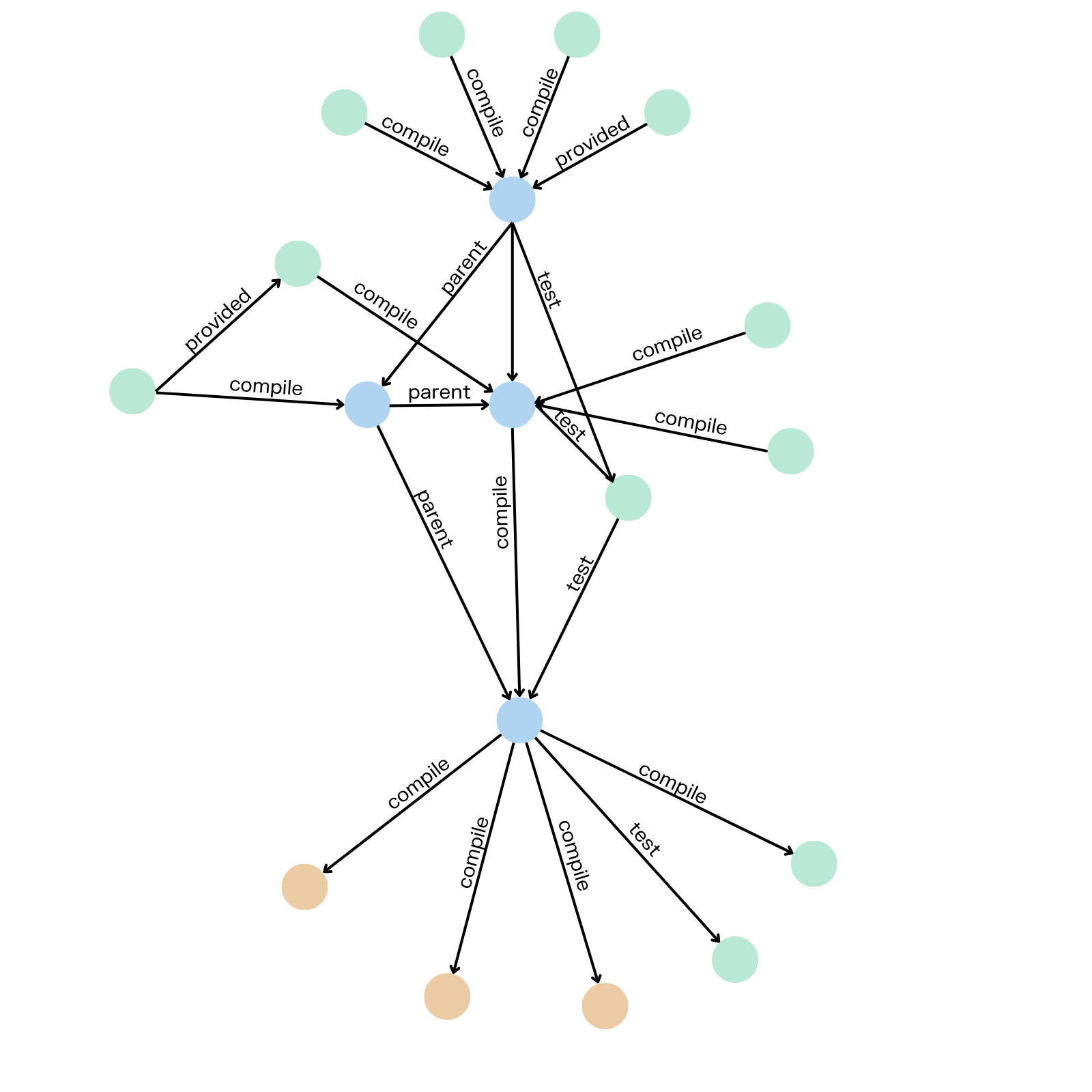
Let's apply this to the dependency graph above.

• To find the shortest chain of dependencies that could cause a test component to fail, you would use BFS.
• To check for circular dependencies (a fatal flaw in a build system), you would use DFS.

---

Conclusion

In this lesson, you implemented the two most fundamental graph traversal algorithms and, more importantly, learned the principles that guide when to use them.

Key Takeaways:

• DFS (Stack/Recursion): Goes deep first. It's great for pathfinding, cycle detection, and exploring exhaustive possibilities (like in puzzles).
• BFS (Queue): Goes wide first, level by level. Its primary strength is finding the shortest path in an unweighted graph.
• Implementation: Both have iterative versions that are structurally similar, differing mainly by the use of a stack (DFS) versus a queue (BFS).
• Complexity: Both are $O(V+E)$ time. The space complexity trade-off depends on the graph's shape (deep and narrow favors BFS, wide and shallow favors DFS).
• The choice is driven by the problem. There is no "better" algorithm; there is only the right tool for the job.

Next Lesson Preview

Now that you have mastered traversing a graph, you're ready to use that skill to solve a classic and highly practical problem. In the next lesson, "Implement topological sort on a Directed Acyclic Graph (DAG) using Kahn's algorithm (BFS-based)," we will use BFS to create a linear ordering of dependent tasks, a core requirement for any scheduler or build system.