Recommended resources
The freely available resources this lesson will direct you to.
Hello! In the previous lesson, you placed an order number in the order-line fact as a degenerate dimension and grouped small transaction classifications in a junk dimension. Both decisions depended on what each value described. A changing attribute adds a second question: should a report about an old order use the attribute’s old value or its current value?
This lesson gives you a way to choose an SCD Type 1, Type 2, or Type 3 policy for each attribute. You’ll trace the effect of each choice on existing fact rows, then apply the policies to an order-line model. Estimated study time: about 40 minutes.
The reporting question comes before the SCD type
Imagine a salesperson assigned to Region A in March and Region B from April onward. Your order-line fact retains sales in both months. If a report groups all those lines by salesperson region, there are two defensible answers:
- Current organization: show both months’ sales under Region B.
- Organization at the time of sale: show March under Region A and later sales under Region B.
Neither is intrinsically correct. The choice depends on the report’s purpose. An SCD policy is the agreement that makes that choice predictable, rather than an ETL behavior discovered after a historical total changes.
Watch the selected portion of Understand Slowly Changing Dimensions by Bryan Cafferky. Focus on the reporting consequence of a region reassignment and on how facts refer to different versions under Type 2.
Understand Slowly Changing Dimensions
In Understand Slowly Changing Dimensions, Bryan Cafferky uses changing customer and organizational attributes to show why an ordinary source-table overwrite can alter historical analysis.
Watch the reporting problem for the historical-region example. Then watch Type 1, Type 2, and Type 3. In the Type 2 portion, notice that successive versions have different dimension keys even though they describe the same person.
The word slowly is conventional, but frequency alone does not select a type. A rare region change may demand exact history; a frequent correction to an unimportant display field may not. Specify the policy per attribute, using the analytical questions the dimension must answer.
Three different promises about history
Read the concise definitions in Kimball Group’s Kimball Dimensional Modeling Techniques. They are useful as a policy reference alongside the video: pay particular attention to what happens to existing fact relationships when Type 2 creates a new surrogate key.
Kimball Dimensional Modeling Techniques
Read Kimball Group’s Kimball Dimensional Modeling Techniques for its compact definitions of Types 1, 2, and 3 and the reporting consequences of each.
On p. 12, find “Slowly Changing Dimension Techniques.” Within its “Type 1: Overwrite,” “Type 2: Add New Row,” and “Type 3: Add New Attribute” subsections, read Types 1 to 3. Stop before “Type 4: Add Mini-Dimension.” Focus on which changes need a new row, which leave fact foreign keys untouched, and why Type 3 offers only a limited alternative view.
Here is the practical distinction you will use throughout the lesson:
| Policy | Change to the dimension | What happens to earlier fact rows? |
|---|---|---|
| Type 1 | Overwrite the attribute in its existing row | Their foreign keys stay the same; reports now see the new value. |
| Type 2 | Close the old version and add a row with a new surrogate key | Their foreign keys stay on the old version; new facts use the new version. |
| Type 3 | Overwrite the main value and retain a designated former value in another column | Their foreign keys stay the same; reports can use either column, but not a complete sequence of past values. |
These are policies for meaning, not just storage recipes. In particular, Type 3 does not become a smaller Type 2 merely because it has a “previous” column.
Type 1: correct or deliberately restate the past
Suppose dim_product contains product_name = 'Adjustible Stand', a misspelling. Correcting it to Adjustable Stand should ordinarily change the label for every report, including reports on old orders. A Type 1 overwrite does that without creating a new product version. The fact rows continue to reference the same product surrogate key.
The same mechanism has a very different effect on a meaningful classification. If you overwrite a salesperson’s region from A to B, all sales tied to that dimension row will now group under B—even sales made while the salesperson worked in A. Type 1 is therefore suitable when the business wants current-state reporting, or when the former value was an error rather than a valid historical state. It is unsuitable when an old classification must remain available for an “as it was then” report.
This also affects stored results outside the base star. An aggregate table or cube grouped by the old region may need to be rebuilt after the overwrite; changing the dimension label alone does not necessarily repair a previously computed regional total. Type 1 is simple to load, but its effect on downstream reporting is not always small.
Type 2: retain the classification that applied to each fact
Now suppose the historical regional assignment does matter. Give each version of the salesperson its own dimension surrogate key while retaining the same source salesperson ID as an attribute:
| salesperson_key | source_salesperson_id | region | valid_from | valid_to | is_current |
|---|---|---|---|---|---|
| 41 | S7 | Region A | 2025-01-01 | 2025-04-01 | false |
| 84 | S7 | Region B | 2025-04-01 | open | true |
For this lesson, the validity convention is start inclusive, end exclusive: the first row is valid from January 1 up to but not including April 1; the second begins on April 1. A load must not find two valid versions, or no version, for a known salesperson at the relevant event time. The current-row indicator is a convenient way to find today’s version; its value must agree with the validity interval.
The accompanying order lines retain different foreign keys:
| order date | salesperson_key | net_amount |
|---|---|---|
| 2025-03-14 | 41 | 100 |
| 2025-05-12 | 84 | 150 |
A region rollup through those keys reports 100 in Region A and 150 in Region B. The source ID S7 identifies the continuing business person; it cannot be the dimension table’s unique primary key when both versions exist. Nor should you join the fact to this dimension on source_salesperson_id alone: each fact would match both versions and its amount could be counted twice.
The image below depicts the same essential distinction for a product. Its source product ID 010 is unchanged, while the old and revised descriptions occupy dimension rows with different surrogate IDs.
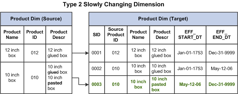
The image labels an old row’s end date with the same calendar date as the new row’s start. That drawing does not specify whether end dates are inclusive. Your implementation must choose and document a boundary convention, such as the half-open intervals used in our table. The image also uses a distant end date for a current row; the table above says “open.” Either representation needs a consistent lookup rule.
Type 2 has a load-time obligation. When a late-arriving March order is loaded in June, “use the current salesperson row” would assign key 84 and misclassify the sale. The load must resolve the version valid on the order’s applicable business date, key 41 in this example. An existing March fact that already references key 41 does not need to be re-keyed simply because April’s version was added. Backdated source corrections require particular care because they can change the intervals and the version appropriate to previously loaded facts.
The date dimension still answers when the order occurred. The salesperson version answers which regional description applied. Both are needed; one does not replace the other.
Type 3: retain a specified alternative, not a timeline
Suppose stakeholders want to compare a customer’s current service tier with the immediately previous tier, but have no requirement to reconstruct every tier change at every past order date. A Type 3 design can hold current_tier and previous_tier in one customer row:
| customer_key | current_tier | previous_tier |
|---|---|---|
| 27 | Gold | Silver |
If the tier next changes to Platinum, an immediate-previous-value policy produces current_tier = Platinum and previous_tier = Gold. The earlier Silver value is gone. You could instead explicitly retain an original tier, but that is a different policy and should be named accordingly.
Because the dimension row and fact foreign keys have not changed, grouping old orders by current_tier categorizes all of that customer’s orders as Platinum. Grouping them by previous_tier categorizes all of them as Gold. Neither column assigns Silver, Gold, and Platinum to the exact periods when those tiers applied. Type 3 offers two chosen perspectives on the same facts, not a time-correct history. If analysts ask for tier-at-purchase reporting after multiple changes, choose Type 2 instead.
Make the choice attribute by attribute
A dimension can have more than one change policy. For example, a salesperson’s corrected display name might be Type 1, while their regional assignment is Type 2. The policy should state what constitutes a correction and what constitutes a real change: a corrected spelling need not create a historical version merely because another attribute in the table uses Type 2.
Before agreeing on a policy, work through these decisions with the people who will use the reports:
- Was the old value ever valid? If it was an error, a Type 1 correction usually expresses the intended truth.
- Must old facts retain their then-current classification? If yes, use Type 2 and specify the business-effective time, version boundaries, and late-fact lookup rule.
- Is a deliberately limited comparison sufficient? If users only need a named original or previous value alongside the current one, Type 3 may fit. State what is lost on the next change.
- Which reports must remain comparable? Record whether historical regional totals should remain “as-was” or be restated to today’s organization. Also identify aggregates that a Type 1 change would invalidate.
Do not apply Type 2 to every field simply to be safe. Excess versions make the dimension harder to load and analyze. Equally, do not choose Type 1 just because the source system exposes only its latest value: if historical assignments matter, you need a reliable way to capture changes and establish when they took effect. Your experience with incremental pipelines is useful here—the availability of change events or snapshots determines how accurately a stated history policy can be delivered.
Conclusion
Type 1 overwrites a value and deliberately changes how existing facts are described. Type 2 creates a new surrogate-keyed version so facts can retain the description applicable at their event time. Type 3 keeps a limited, explicitly named alternative value but cannot reconstruct a full timeline. Choose among them for each changing attribute by asking what an old fact must mean in a future report.
In the next lesson, you’ll carry these decisions across business processes: a bus matrix and conformed dimensions must give shared attributes—and their history—consistent meanings in more than one fact table.