Partial Derivatives and Total Differentials

Recommended resources

The freely available resources this lesson will direct you to.

Hello! This course develops mathematical tools that recur throughout higher physics, then uses them in physical and quantum-mechanical settings. We begin with a basic question: how does a quantity change when it depends on more than one input? In this lesson, you will compute partial derivatives, combine them into a total differential, and use that differential to estimate a small change in a physical quantity.

Changing one input at a time

Suppose $f (x, y)$ depends on two independent variables. In single-variable calculus, a derivative measures the effect of changing the input. Here we can ask two distinct questions: what happens when $x$ changes while $y$ stays fixed, and what happens when $y$ changes while $x$ stays fixed? Their answers are the partial derivatives $f_{x}$ and $f_{y}$ .

At a point $(a, b)$ , the definitions are

f_{x} (a, b) = h \to 0 lim \frac{f ( a + h , b ) - f ( a , b )}{h}, f_{y} (a, b) = k \to 0 lim \frac{f ( a , b + k ) - f ( a , b )}{k} .

Notice what does not change in each limit: $b$ is fixed in the first, and $a$ is fixed in the second. In practice, this means treating every other independent variable as a constant and applying ordinary differentiation rules.

4.3 Partial Derivatives - Calculus Volume 3

Read OpenStax’s introduction to partial derivatives for the limit definitions and the practical rule for calculating them.

Under “Derivatives of a Function of Two Variables,” begin with definitions and notation, stopping before Example 4.14. Then, immediately after Checkpoint 4.12, read the calculation rule and Example 4.15. Focus on which variables are held fixed; you do not need to work the checkpoints now.

For example, let

f (x, y) = x^{2} y + 3 y^{2} .

Holding $y$ fixed makes it a coefficient when differentiating $x^{2} y$ . Holding $x$ fixed makes $x^{2}$ a coefficient when differentiating that same term. Thus

f_{x} (x, y) = 2 x y, f_{y} (x, y) = x^{2} + 6 y .

At $(2, 1)$ , these rates are $f_{x} (2, 1) = 4$ and $f_{y} (2, 1) = 10$ . The function’s response depends on which input you vary.

The same method works with more inputs. For $F (x, y, z) = x^{2} z + sin y$ , there are three first partial derivatives:

F_{x} = 2 x z, F_{y} = cos y, F_{z} = x^{2} .

Each calculation holds the other two variables fixed.

From slopes to a tangent plane

If $z = f (x, y)$ , its graph is a surface. Fixing $y = b$ cuts a curve through that surface. The slope of this curve at $(a, b, f (a, b))$ is $f_{x} (a, b)$ ; the corresponding slice with $x = a$ has slope $f_{y} (a, b)$ .

The green curve is the slice of $z=f(x,y)$ obtained by holding $y=b$. Its tangent-line slope at the marked point is $f_x(a,b)$.

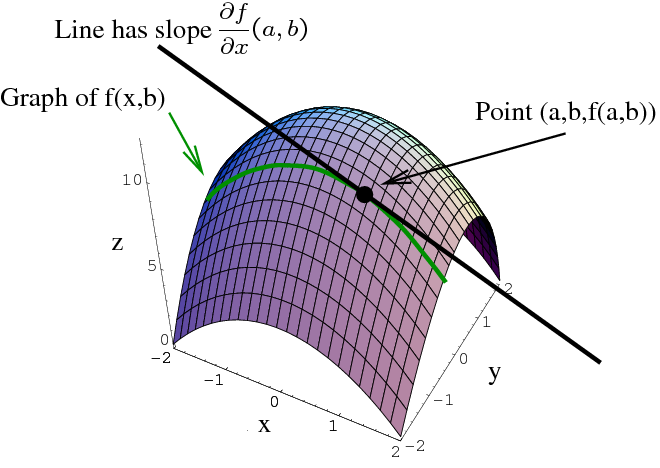
When the surface is sufficiently smooth, these two slopes specify its tangent plane at the point. The plane gives a linear approximation near $(a, b)$ :

L (x, y) = f (a, b) + f_{x} (a, b) (x - a) + f_{y} (a, b) (y - b) .

This is the multivariable counterpart of approximating a curve by its tangent line. The plane agrees with the surface at the base point and captures its first-order change in both input directions.

The translucent plane is tangent to the orange surface at the marked point. Tangent lines to curves on the surface through that point lie in the tangent plane.

The total differential: a predicted small change

Let the inputs change by $d x$ and $d y$ . The total differential is the change predicted by the tangent plane:

df = f_{x} (x, y) d x + f_{y} (x, y) d y .

For independently chosen input changes, we set $d x = Δ x$ and $d y = Δ y$ . The actual output change, however, is

Δ f = f (x + Δ x, y + Δ y) - f (x, y) .

In general, $Δ f$ is not exactly equal to $df$ : the surface can bend away from its tangent plane. For sufficiently small input changes at a differentiable point, $df$ approximates $Δ f$ .

Watch the following short lecture segment for the distinction between an actual change and a differential. It also connects the two-input formula to the single-variable tangent-line idea.

Lec 11: Differentials; chain rule | MIT 18.02 Multivariable Calculus, Fall 2007

Watch “Differentials; chain rule” from MIT OpenCourseWare for its introduction to the total differential. Stop before the lecture turns to the chain rule, which is the next lesson’s topic.

Watch the setup for the connection to single-variable differentials, followed by actual versus predicted change. Focus on why the differential uses the local linear approximation rather than claiming to equal every finite change.

OpenStax develops the tangent-plane approximation and states when it is valid. The essential condition is differentiability: near the base point, the error in the linear prediction must become small compared with the size of the input change. Continuous first partial derivatives in a neighborhood are a useful sufficient condition. Merely finding two partial derivatives at one point is not enough to guarantee a good tangent-plane approximation there.

4.4 Tangent Planes and Linear Approximations

Read OpenStax’s account of how a tangent plane leads to a linear approximation and a total differential. Pay particular attention to the distinction between a condition for differentiability and simply calculating partial derivatives.

In “Linear Approximations,” begin at the tangent-plane approximation, continuing through Example 4.23. In “Differentiability,” read the error definition; then find Theorem 4.7 and read the continuity criterion. Finally, in “Differentials,” start where the text extends the single-variable idea and read the total differential. Focus on its formula and how it estimates a change; leave the later three-variable definition and exercises for another time.

For a differentiable function, the precise statement behind “small change” is

f (a + h, b + k) = f (a, b) + f_{x} (a, b) h + f_{y} (a, b) k + r (h, k),

where the remainder satisfies

\frac{r ( h , k )}{h ^{2} + k ^{2}} ⟶ 0 as (h, k) ⟶ (0, 0) .

The differential is the two-term linear part. This explains both its usefulness and its limit: it captures the leading response near the chosen point, not necessarily the exact response to a finite step.

Computing and using a differential

Return to $f (x, y) = x^{2} y + 3 y^{2}$ . Since its partial derivatives are $2 x y$ and $x^{2} + 6 y$ , its total differential is

df = 2 x y d x + (x^{2} + 6 y) d y .

At $(2, 1)$ , this becomes $df = 4 d x + 10 d y$ . If $x$ increases by $0.01$ and $y$ decreases by $0.02$ , the predicted change is

df = 4 (0.01) + 10 (- 0.02) = - 0.16.

Because $f (2, 1) = 7$ , the corresponding linear estimate is $f (2.01, 0.98) \approx 6.84$ . Direct evaluation gives $f (2.01, 0.98) = 6.840498$ , so the exact change is $- 0.159502$ . The small difference between these changes is the part the tangent plane does not capture.

A physical example makes the roles of the inputs clearer. Kinetic energy as a function of mass $m$ and speed $v$ is $K (m, v) = \frac{1}{2} m v^{2}$ . Treating the two inputs independently gives

K_{m} = \frac{1}{2} v^{2}, K_{v} = m v, d K = \frac{1}{2} v^{2} d m + m v d v .

The first term estimates the energy change attributable to a small mass change with speed held fixed; the second does the same for a speed change with mass held fixed. The total differential combines both contributions when both inputs vary. With three or more independent variables, you use the same rule: compute one first partial derivative per input and multiply each by that input’s differential.

Looking ahead

A partial derivative measures change while the other inputs are fixed. The total differential combines those separate rates into one local, linear prediction for simultaneous input changes. Keep the distinction between $df$ and the exact change $Δ f$ in view: it will matter whenever a physical model is approximated near a chosen state.

Next, you will study what happens when the inputs are themselves functions of other variables. That leads to the multivariable chain rule and Jacobian matrices.