Applying the Multivariable Chain Rule with Jacobian Matrices

Hello! Last lesson, you used partial derivatives to predict how a function changes when its inputs change independently. Now suppose those inputs depend on other variables. A quantity might depend on position, for example, while position depends on time. The multivariable chain rule accounts for every route through which a change can reach the quantity you care about.

In this lesson, you will arrange partial derivatives into Jacobian matrices and multiply those matrices to differentiate composite functions. This notation will be useful whenever higher physics calls for a change of coordinates, a trajectory through a field, or several coupled quantities.

---

The Jacobian gathers the partial derivatives

Suppose a function takes two inputs and produces two outputs:

$$\mathbf{g}(x_1,x_2)=\left(\begin{array}{c}{g}_1(x_1,x_2)\\ g_2(x_1,x_2)\end{array}\right).$$

There are four first partial derivatives: each output can respond to either input. We arrange them with outputs as rows and inputs as columns:

$$J_{\mathbf{g}}(x_1,x_2)=\left(\begin{array}{cc}\frac{\partial g_1}{\partial x_1}& \frac{\partial g_1}{\partial x_2}\\ \frac{\partial g_2}{\partial x_1}& \frac{\partial g_2}{\partial x_2}\end{array}\right).$$

The Jacobian is the vector-valued counterpart of the total differential from last lesson. Near a point, it predicts the change in all outputs caused by a small input change:

$$d\mathbf{g}=J_{\mathbf{g}}d\mathbf{x},d\mathbf{x}=\left(\begin{array}{c}d{x}_1\\ d{x}_2\end{array}\right).$$

Watch the short portion of The Jacobian Matrix – Explained by DataMListic for a visual introduction to why the derivatives occupy these particular rows and columns.

For a function with $n$ inputs and $m$ outputs, its Jacobian has $m$ rows and $n$ columns. A scalar-valued function therefore has a one-row Jacobian. Keeping track of these dimensions is more than bookkeeping: it helps catch incorrect chain-rule formulas.

---

Why Jacobians multiply

Let $\mathbf{u}=\mathbf{g}(\mathbf{x})$ be a set of intermediate variables, and let $\mathbf{z}=\mathbf{F}(\mathbf{u})$ be the final outputs. From the local linear approximations,

$$d\mathbf{u}=J_{\mathbf{g}}(\mathbf{x})d\mathbf{x},d\mathbf{z}=J_{\mathbf{F}}(\mathbf{u})d\mathbf{u}.$$

Substituting the first relation into the second gives the Jacobian chain rule:

$$J_{\mathbf{F}\circ \mathbf{g}}(\mathbf{x})=J_{\mathbf{F}}(\mathbf{g}(\mathbf{x}))J_{\mathbf{g}}(\mathbf{x}).$$

The evaluation points matter. Differentiate $\mathbf{F}$ with respect to its intermediate inputs, then evaluate that Jacobian at $\mathbf{u}=\mathbf{g}(\mathbf{x})$. Differentiate $\mathbf{g}$ with respect to the original inputs and evaluate it at $\mathbf{x}$.

If $\mathbf{x}$ has $n$ components, $\mathbf{u}$ has $m$, and $\mathbf{z}$ has $p$, the multiplication has dimensions

$$\underset{J_{\mathbf{F}}}{\underbrace{p\times m}}\underset{J_{\mathbf{g}}}{\underbrace{m\times n}}=\underset{J_{\mathbf{F}\circ \mathbf{g}}}{\underbrace{p\times n}}.$$

Matrix multiplication is generally not commutative, so these dimensions also help establish the correct order.

The University of Toronto’s 2.3 The Chain Rule presents the general formula, then specializes it to a scalar output and to a function evaluated along a one-parameter path. Read those parts now; you can leave its examples and optional proof for later.

Here is that entry written explicitly. If the intermediate components are $g_i$ and the final components are $F_k$, then

$$\frac{\partial (F_k\circ \mathbf{g})}{\partial x_j}(\mathbf{x})=\sum _{i=1}^m\frac{\partial F_k}{\partial u_i}(\mathbf{g}(\mathbf{x}))\frac{\partial g_i}{\partial x_j}(\mathbf{x}).$$

Each term represents one intermediate variable through which $x_j$ affects $F_k$. The matrix product collects those terms for every output and every input at once.

---

Follow the paths, then calculate

For a scalar output $h(u_1,u_2)$, the Jacobian $J_h$ is a row. The diagram below shows two intermediate variables, each depending on both original inputs. The two colored routes from $x_1$ to $h$ contribute separate terms to the derivative with respect to $x_1$; the routes from $x_2$ work the same way.

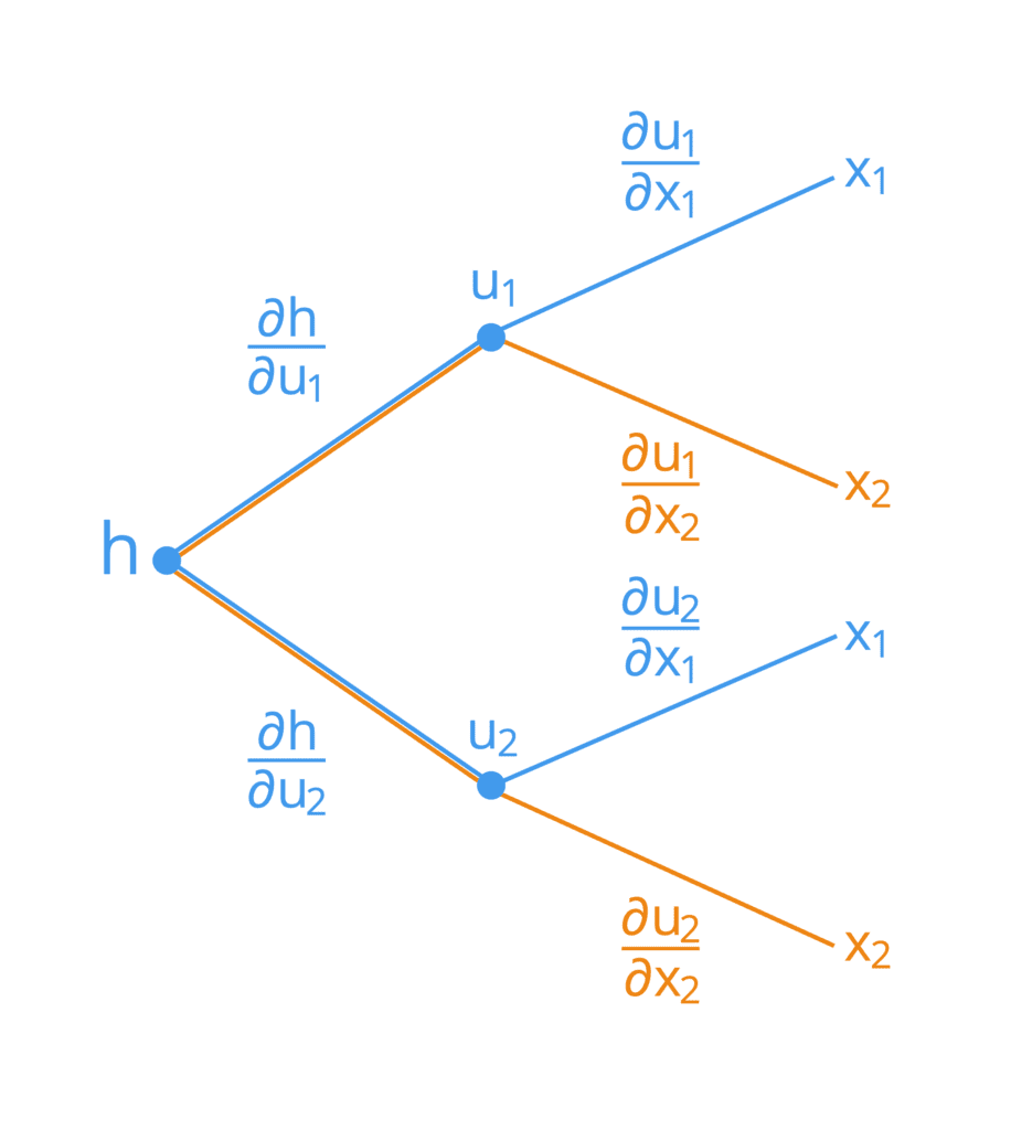
Consider the concrete functions

$$h(u_1,u_2)=u_1^2+3u_2,\mathbf{g}(x_1,x_2)=\left(\begin{array}{c}{x}_1+x_2^2\\ x_1{x}_2\end{array}\right).$$

Before substituting for $u_1$ and $u_2$, compute the two Jacobians:

$$J_h(u_1,u_2)=\left(\begin{array}{cc}2u_1& 3\end{array}\right),J_{\mathbf{g}}(x_1,x_2)=\left(\begin{array}{cc}1& 2x_2\\ x_2& x_1\end{array}\right).$$

Their product is the complete derivative of $h\circ \mathbf{g}$:

$$J_{h\circ \mathbf{g}}(x_1,x_2)=\left(\begin{array}{cc}2(x_1+x_2^2)+3x_2& 4x_2(x_1+x_2^2)+3x_1\end{array}\right).$$

For instance, at $(x_1,x_2)=(1,2)$, the intermediate point is $(u_1,u_2)=(5,2)$. Evaluating each Jacobian at its appropriate point gives

$$J_{h\circ \mathbf{g}}(1,2)=\left(\begin{array}{cc}10& 3\end{array}\right)\left(\begin{array}{cc}1& 4\\ 2& 1\end{array}\right)=\left(\begin{array}{cc}16& 43\end{array}\right).$$

Thus, near $(1,2)$, a small change in $x_1$ alone produces approximately $16d{x}_1$ change in the output; a small change in $x_2$ alone produces approximately $43d{x}_2$. As a check, substituting first gives $h\circ \mathbf{g}=(x_1+x_2^2{)}^2+3x_1{x}_2$, whose two partial derivatives agree with the product.

A common source of errors is using the same notation for a partial derivative of $h$, with its intermediate inputs held independent, and a partial derivative of the composite, whose intermediate inputs now vary with $x_1$ or $x_2$. Naming both functions, as $h$ and $h\circ \mathbf{g}$, keeps those operations distinct.

---

Multiple outputs and physical trajectories

The matrix rule is not limited to a scalar final result. Suppose we retain the same $\mathbf{g}$, but want two outputs:

$$\mathbf{F}(u_1,u_2)=\left(\begin{array}{c}{u}_1^2+3u_2\\ u_1-u_2^2\end{array}\right).$$

Now $J_{\mathbf{F}}$ has two rows. At the intermediate point $(5,2)$,

$$J_{\mathbf{F}}(5,2)=\left(\begin{array}{cc}10& 3\\ 1& -4\end{array}\right).$$

Consequently, at $(x_1,x_2)=(1,2)$,

$$J_{\mathbf{F}\circ \mathbf{g}}(1,2)=\left(\begin{array}{cc}10& 3\\ 1& -4\end{array}\right)\left(\begin{array}{cc}1& 4\\ 2& 1\end{array}\right)=\left(\begin{array}{cc}16& 43\\ -7& 0\end{array}\right).$$

The first row reproduces the scalar calculation. The second row gives the sensitivities of the other output to the same two original inputs. One multiplication has handled both outputs without changing the rule.

A particularly useful physical case has one time input. Suppose a particle follows a planar path $\mathbf{r}(t)=(x(t),y(t))$, while a scalar field $U(x,y)$ assigns a value to each position. Here $J_{\mathbf{r}}$ is a two-entry column, and $J_U$ is a two-entry row:

$$\frac{d}{dt}U(x(t),y(t))={\left(\begin{array}{cc}{U}_x& U_y\end{array}\right)}_{(x(t),y(t))}\left(\begin{array}{c}{x}^{\prime }(t)\\ y^{\prime }(t)\end{array}\right)=U_x{x}^{\prime }+U_y{y}^{\prime }.$$

This is the last lesson’s total differential applied when the input changes are determined by a path, rather than chosen independently. For example, take $U(x,y)=\frac{k}{2}(x^2+y^2)$ and a circular path $x(t)=R\cos (\omega t)$, $y(t)=R\sin (\omega t)$. Since $U_x=kx$ and $U_y=ky$, the chain rule gives $dU/dt=k(x{x}^{\prime }+y{y}^{\prime })=0$. The field value is constant on that path, even though both coordinates are changing.

---

A coordinate-change example

The same calculation applies when the original inputs are coordinates rather than time. In polar coordinates, $x=r\cos \theta$ and $y=r\sin \theta$. If $\varphi (r,\theta )=f(x(r,\theta ),y(r,\theta ))$, the Jacobian chain rule determines both partial derivatives of $\varphi$ in one product.

Read “Example 1: Polar coordinates” in the same University of Toronto notes. It provides a useful model for checking which variables are held fixed in each derivative.

In particular,

$$J_{\mathbf{g}}(r,\theta )=\left(\begin{array}{cc}\cos \theta & -r\sin \theta \\ \sin \theta & r\cos \theta \end{array}\right),J_{\varphi }={\left(\begin{array}{cc}{f}_x& f_y\end{array}\right)}_{(r\cos \theta ,r\sin \theta )}{J}_{\mathbf{g}}.$$

The first column of the product is $\partial \varphi /\partial r$; the second is $\partial \varphi /\partial \theta$. In both, $f_x$ and $f_y$ must be evaluated at the corresponding Cartesian point, not at $(r,\theta )$. Coordinate transformations recur throughout physics; for now, the central skill is to identify the composed functions and multiply their Jacobians in the right order.

---

Looking ahead

A Jacobian records the first-order response of every output to every input. For a composition, evaluate the outer Jacobian at the intermediate point and multiply it by the inner Jacobian. Matrix dimensions, evaluation points, and the distinction between an intermediate function and its composite are your most reliable checks.

Next, you will use the gradient to find how a scalar field changes in a specified direction. The path calculation above already hints at the connection: it pairs the field’s partial derivatives with the way position is changing.