Angular Momentum: Commutation Relations and Eigenvalues

Hello! Welcome to the second module of our course, "Advanced Angular Momentum and Spin."

In our last lesson, which concluded the module on symmetries, we saw the power of the Wigner-Eckart theorem in predicting selection rules for atomic transitions. That theorem relied on the properties of angular momentum eigenstates, denoted $|j,m⟩$, and concepts like Clebsch-Gordan coefficients. We used these tools without proving where they came from. Now, we will build that entire theoretical structure from the ground up.

This lesson addresses the first learning outcome of this module: to derive the general theory of angular momentum from commutation relations and determine the eigenvalue spectrum. We will start with a purely algebraic definition of angular momentum and, through a beautiful and powerful method involving "ladder operators," deduce the famous quantization rules for the quantum numbers $j$ and $m$. This derivation is a cornerstone of quantum theory because its results apply universally to orbital angular momentum, spin, and the total angular momentum of any isolated system.

1. The Algebraic Definition of Angular Momentum

In quantum mechanics, any set of three Hermitian operators ${\hat{J}}_x,{\hat{J}}_y,{\hat{J}}_z$ is defined as an angular momentum operator if its components satisfy the following cyclic commutation relations:

$$[{\hat{J}}_x,{\hat{J}}_y]=i\hslash {\hat{J}}_z,[{\hat{J}}_y,{\hat{J}}_z]=i\hslash {\hat{J}}_x,[{\hat{J}}_z,{\hat{J}}_x]=i\hslash {\hat{J}}_y$$

This can be written compactly using the Levi-Civita symbol ${ϵ}_{ijk}$ as $[{\hat{J}}_i,{\hat{J}}_j]=i\hslash {\sum }_k{ϵ}_{ijk}{\hat{J}}_k$.

Since the components do not commute with each other, they are incompatible observables; we cannot know the values of $J_x$, $J_y$, and $J_z$ simultaneously. We need to find a set of commuting observables. Let's define the total angular momentum squared operator:

$${\hat{J}}^2={\hat{J}}_x^2+{\hat{J}}_y^2+{\hat{J}}_z^2$$

It is a crucial fact that ${\hat{J}}^2$ commutes with each of its components:

$$[{\hat{J}}^2,{\hat{J}}_i]=0\text{for }i\in \{x,y,z\}$$

Because ${\hat{J}}^2$ and, say, ${\hat{J}}_z$ commute, they form a Complete Set of Commuting Observables (CSCO) for this problem. This guarantees that we can find a basis of simultaneous eigenvectors for both operators. Our goal is to find the eigenvalues of these operators.

Let's label our common eigenvectors by their eigenvalues, which we'll call $\lambda$ and $\mu$ for now:

$${\hat{J}}^2|\lambda ,\mu ⟩=\lambda |\lambda ,\mu ⟩$$ $${\hat{J}}_z|\lambda ,\mu ⟩=\mu |\lambda ,\mu ⟩$$

The following resource provides a formal setup of these initial commutation relations and the eigenvalue problem.

2. The Ladder Operator Method

To find the allowed values of $\lambda$ and $\mu$, we'll use an algebraic technique known as the ladder operator method, which you might have seen when solving the quantum harmonic oscillator.

We define two non-Hermitian ladder operators:

$${\hat{J}}_{+}={\hat{J}}_x+i{\hat{J}}_y(\text{raising operator})$$ $${\hat{J}}_{-}={\hat{J}}_x-i{\hat{J}}_y(\text{lowering operator})$$

Note that ${\hat{J}}_{+}^{†}={\hat{J}}_{-}$.

The power of these operators comes from their commutation relations with ${\hat{J}}_z$ and ${\hat{J}}^2$. Through straightforward algebra, one can show:

1. $[{\hat{J}}_z,{\hat{J}}_{\pm }]=\pm \hslash {\hat{J}}_{\pm }$
2. $[{\hat{J}}^2,{\hat{J}}_{\pm }]=0$

Let's see what these imply. If we act on our eigenstate $|\lambda ,\mu ⟩$ with ${\hat{J}}_{\pm }$, what do we get?
For the ${\hat{J}}^2$ eigenvalue:

$${\hat{J}}^2({\hat{J}}_{\pm }|\lambda ,\mu ⟩)={\hat{J}}_{\pm }{\hat{J}}^2|\lambda ,\mu ⟩={\hat{J}}_{\pm }(\lambda |\lambda ,\mu ⟩)=\lambda ({\hat{J}}_{\pm }|\lambda ,\mu ⟩)$$

The new state ${\hat{J}}_{\pm }|\lambda ,\mu ⟩$ is also an eigenstate of ${\hat{J}}^2$ with the same eigenvalue $\lambda$.

For the ${\hat{J}}_z$ eigenvalue:

$${\hat{J}}_z({\hat{J}}_{\pm }|\lambda ,\mu ⟩)=({\hat{J}}_{\pm }{\hat{J}}_z\pm \hslash {\hat{J}}_{\pm })|\lambda ,\mu ⟩={\hat{J}}_{\pm }(\mu |\lambda ,\mu ⟩)\pm \hslash ({\hat{J}}_{\pm }|\lambda ,\mu ⟩)=(\mu \pm \hslash )({\hat{J}}_{\pm }|\lambda ,\mu ⟩)$$

The new state ${\hat{J}}_{\pm }|\lambda ,\mu ⟩$ is an eigenstate of ${\hat{J}}_z$ with a new eigenvalue $\mu \pm \hslash$.

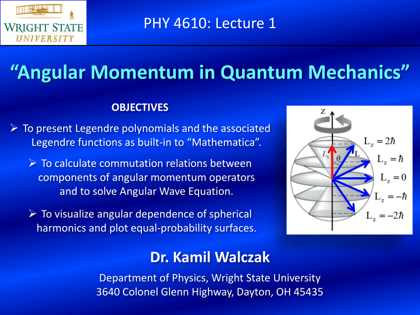
This is why they are called ladder operators: they move us up or down a "ladder" of ${\hat{J}}_z$ eigenvalues, all while keeping the ${\hat{J}}^2$ eigenvalue fixed.

The following video provides a very detailed, step-by-step walkthrough of setting up the operators and deriving the commutation relations and their consequences.

3. Bounding the Ladder and Finding the Spectrum

We have a ladder of states, but can it extend forever? No. We can show that the eigenvalues must satisfy the inequality $\lambda \ge {\mu }^2$. This is because:

$$⟨{\hat{J}}^2⟩=⟨{\hat{J}}_x^2+{\hat{J}}_y^2+{\hat{J}}_z^2⟩$$

Since ${\hat{J}}_x$ and ${\hat{J}}_y$ are Hermitian, $⟨{\hat{J}}_x^2⟩\ge 0$ and $⟨{\hat{J}}_y^2⟩\ge 0$. Therefore, for any eigenstate $|\lambda ,\mu ⟩$:

$$\lambda =⟨{\hat{J}}^2⟩\ge ⟨{\hat{J}}_z^2⟩={\mu }^2$$

Since $\mu$ cannot increase or decrease infinitely, there must be a "top rung" and a "bottom rung" of the ladder.

• There exists a maximum eigenvalue ${\mu }_{max}$ and a corresponding state $|\lambda ,{\mu }_{max}⟩$ such that applying the raising operator gives zero: ${\hat{J}}_{+}|\lambda ,{\mu }_{max}⟩=0$.
• There exists a minimum eigenvalue ${\mu }_{min}$ and a corresponding state $|\lambda ,{\mu }_{min}⟩$ such that applying the lowering operator gives zero: ${\hat{J}}_{-}|\lambda ,{\mu }_{min}⟩=0$.

Now we use this to find $\lambda$. We need the following operator identities, which can be derived by expanding the definitions of ${\hat{J}}_{\pm }$:

$${\hat{J}}_{-}{\hat{J}}_{+}={\hat{J}}^2-{\hat{J}}_z^2-\hslash {\hat{J}}_z$$ $${\hat{J}}_{+}{\hat{J}}_{-}={\hat{J}}^2-{\hat{J}}_z^2+\hslash {\hat{J}}_z$$

Applying the first identity to the top state $|\lambda ,{\mu }_{max}⟩$:

$${\hat{J}}_{-}{\hat{J}}_{+}|\lambda ,{\mu }_{max}⟩=({\hat{J}}^2-{\hat{J}}_z^2-\hslash {\hat{J}}_z)|\lambda ,{\mu }_{max}⟩=0$$ $$(\lambda -{\mu }_{max}^2-\hslash {\mu }_{max})|\lambda ,{\mu }_{max}⟩=0⟹\lambda ={\mu }_{max}({\mu }_{max}+\hslash )$$

Applying the second identity to the bottom state $|\lambda ,{\mu }_{min}⟩$:

$${\hat{J}}_{+}{\hat{J}}_{-}|\lambda ,{\mu }_{min}⟩=({\hat{J}}^2-{\hat{J}}_z^2+\hslash {\hat{J}}_z)|\lambda ,{\mu }_{min}⟩=0$$ $$(\lambda -{\mu }_{min}^2+\hslash {\mu }_{min})|\lambda ,{\mu }_{min}⟩=0⟹\lambda ={\mu }_{min}({\mu }_{min}-\hslash )$$

Equating the two expressions for $\lambda$ gives ${\mu }_{max}({\mu }_{max}+\hslash )={\mu }_{min}({\mu }_{min}-\hslash )$. This quadratic equation has two solutions: ${\mu }_{max}={\mu }_{min}-\hslash$ (which is impossible, since max must be greater than min) and:

$${\mu }_{max}=-{\mu }_{min}$$

The ladder is symmetric about zero!

Furthermore, we must be able to get from the bottom rung to the top rung in some integer number of steps, let's say $N$. Each step increases the eigenvalue by $\hslash$.

$${\mu }_{max}={\mu }_{min}+N\hslash$$

Substituting ${\mu }_{min}=-{\mu }_{max}$, we get $2{\mu }_{max}=N\hslash$, or ${\mu }_{max}=\frac{N}{2}\hslash$.

It is conventional to define a new number, $j=N/2$. This number $j$ is called the angular momentum quantum number. Since $N$ is an integer ($0,1,2,\dots$), $j$ can be an integer or a half-integer:

$$j=0,\frac{1}{2},1,\frac{3}{2},2,\dots$$

With this, ${\mu }_{max}=j\hslash$. The eigenvalues of ${\hat{J}}_z$, which we denote $\mu =m\hslash$, must then range from $-j\hslash$ to $+j\hslash$ in steps of $\hslash$. This means the magnetic quantum number $m$ takes on $2j+1$ values:

$$m=-j,-j+1,\dots ,j-1,j$$

Finally, we find the eigenvalue $\lambda$ of ${\hat{J}}^2$ by substituting ${\mu }_{max}=j\hslash$ back into our formula for $\lambda$:

$$\lambda =(j\hslash )(j\hslash +\hslash )=j(j+1){\hslash }^2$$

This completes the derivation! The following resource presents this final part of the argument very concisely.

Test your understanding!

A quantum system is in a state with total angular momentum quantum number $j=\frac{5}{2}$.

1. What is the eigenvalue of the ${\hat{J}}^2$ operator for this state?
2. What are the possible eigenvalues of the ${\hat{J}}_z$ operator? How many distinct $m$ states are there?

Show answer

1. The eigenvalue of ${\hat{J}}^2$ is $\lambda =j(j+1){\hslash }^2$. With $j=5/2$, we have: $$\lambda =\frac{5}{2}\left(\frac{5}{2}+1\right){\hslash }^2=\frac{5}{2}\cdot \frac{7}{2}{\hslash }^2=\frac{35}{4}{\hslash }^2$$
2. The possible values for the magnetic quantum number $m$ range from $-j$ to $+j$ in integer steps. For $j=5/2$, the possible values of $m$ are: $$m=-\frac{5}{2},-\frac{3}{2},-\frac{1}{2},\frac{1}{2},\frac{3}{2},\frac{5}{2}$$ The possible eigenvalues of ${\hat{J}}_z$ are $m\hslash$, i.e., $-\frac{5}{2}\hslash ,-\frac{3}{2}\hslash ,\dots ,\frac{5}{2}\hslash$.
   There are $2j+1=2(5/2)+1=6$ distinct $m$ states.

Conclusion

In this lesson, we have accomplished something remarkable. Starting only from the commutation relations that define angular momentum, we have derived its entire eigenvalue spectrum through pure algebra.

Key Takeaways:

• Angular momentum is defined by the commutation relation $[{\hat{J}}_i,{\hat{J}}_j]=i\hslash {ϵ}_{ijk}{\hat{J}}_k$.
• Because $[{\hat{J}}^2,{\hat{J}}_z]=0$, we can find their common eigenstates, which we label $|j,m⟩$.
• The ladder operators ${\hat{J}}_{\pm }={\hat{J}}_x\pm i{\hat{J}}_y$ move between states of different $m$ but the same $j$.
• The existence of maximum and minimum $m$ values for a given $j$ forces the quantization of the spectrum.
• The eigenvalue of ${\hat{J}}^2$ is ${\hslash }^{2}j(j+1)$, where $j$ can be an integer or half-integer ($0,1/2,1,\dots$).
• The eigenvalue of ${\hat{J}}_z$ is $\hslash m$, where $m$ takes one of the $2j+1$ values from $-j$ to $+j$ in integer steps.

The generality of this result is its greatest strength. It explains the integer quantum numbers ($l,m_l$) of orbital angular momentum and provides the foundation for the half-integer quantum numbers ($s,m_s$) of spin, which has no classical analogue.

Preview of the next lesson:
We have now formally defined the basis states $|j,m⟩$. A natural next question is: how do these states transform when the physical system is rotated? Answering this will lead us to construct the matrix representation of the rotation operator in this basis, known as the Wigner D-matrices. This will be our next topic.